

E1C02 09/14/2010
13:35:19 Page 64
infinitesimal. This means that the coefficients A n and B n become continuous functions of frequency
and can be expressed as A(v) and B(v) where
A v
ð Þ ¼
ð 1
À1
y t
ð Þcos vtdt
B v
ð Þ ¼
ð 1
À1
y t
ð Þsin vtdt
ð2:26Þ
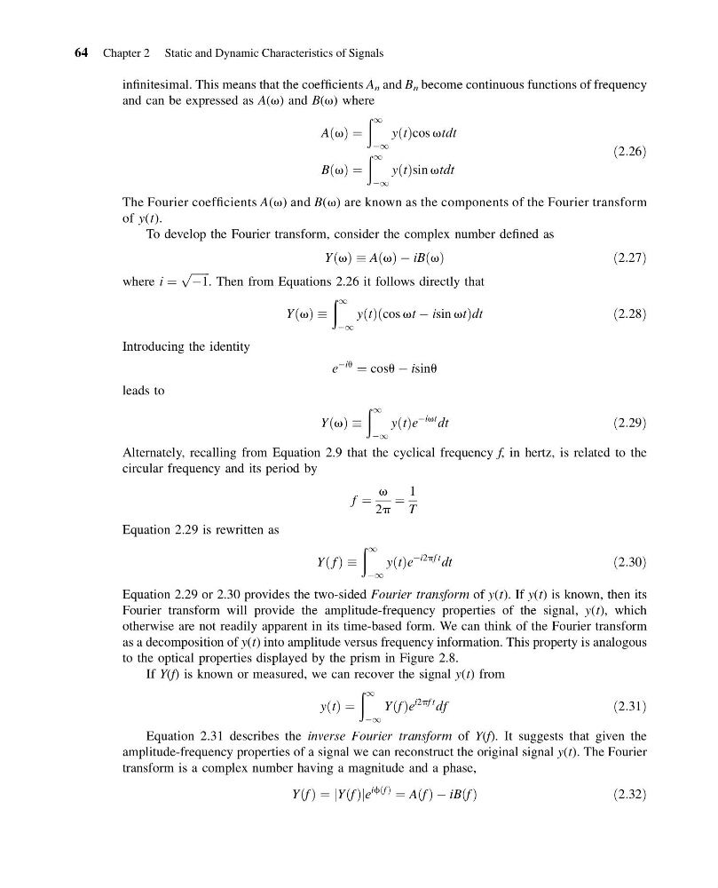
The Fourier coefficients A(v) and B(v) are known as the components of the Fourier transform
of y(t).
To develop the Fourier transform, consider the complex number defined as
Y v
ð Þ A v
ð Þ À iB v
ð Þ
ð2:27Þ
where i ¼
ffiffiffiffiffiffi ffi
À1
p
. Then from Equations 2.26 it follows directly that
Y v
ð Þ
ð 1
À1
y t
ð Þ cos vt À isin vt
ð
Þ dt
ð2:28Þ
Introducing the identity
e
Àiu
¼ cosu À isinu
leads to
Y v
ð Þ
ð 1
À1
y t
ð Þe
Àivt
dt
ð2:29Þ
Alternately, recalling from Equation 2.9 that the cyclical frequency f, in hertz, is related to the
circular frequency and its period by
f ¼
v
2p
¼
1
T
Equation 2.29 is rewritten as
Y f
ð Þ
ð 1
À1
y t
ð Þe
Ài2pf t
dt
ð2:30Þ
Equation 2.29 or 2.30 provides the two-sided Fourier transform of y(t). If y(t) is known, then its
Fourier transform will provide the amplitude-frequency properties of the signal, y(t), which
otherwise are not readily apparent in its time-based form. We can think of the Fourier transform
as a decomposition of y(t) into amplitude versus frequency information. This property is analogous
to the optical properties displayed by the prism in Figure 2.8.
If Y(f) is known or measured, we can recover the signal y(t) from
y t
ð Þ ¼
ð 1
À1
Y f
ð Þe
i2pf t
df
ð2:31Þ
Equation 2.31 describes the inverse Fourier transform of Y(f). It suggests that given the
amplitude-frequency properties of a signal we can reconstruct the original signal y(t). The Fourier
transform is a complex number having a magnitude and a phase,
Y f
ð Þ ¼ jY fÞj
ð e
if f
ð Þ
¼ A f
ð Þ À iB f
ð Þ
ð2:32Þ
64 Chapter 2 Static and Dynamic Characteristics of Signals
13:35:19 Page 64
infinitesimal. This means that the coefficients A n and B n become continuous functions of frequency
and can be expressed as A(v) and B(v) where
A v
ð Þ ¼
ð 1
À1
y t
ð Þcos vtdt
B v
ð Þ ¼
ð 1
À1
y t
ð Þsin vtdt
ð2:26Þ
The Fourier coefficients A(v) and B(v) are known as the components of the Fourier transform
of y(t).
To develop the Fourier transform, consider the complex number defined as
Y v
ð Þ A v
ð Þ À iB v
ð Þ
ð2:27Þ
where i ¼
ffiffiffiffiffiffi ffi
À1
p
. Then from Equations 2.26 it follows directly that
Y v
ð Þ
ð 1
À1
y t
ð Þ cos vt À isin vt
ð
Þ dt
ð2:28Þ
Introducing the identity
e
Àiu
¼ cosu À isinu
leads to
Y v
ð Þ
ð 1
À1
y t
ð Þe
Àivt
dt
ð2:29Þ
Alternately, recalling from Equation 2.9 that the cyclical frequency f, in hertz, is related to the
circular frequency and its period by
f ¼
v
2p
¼
1
T
Equation 2.29 is rewritten as
Y f
ð Þ
ð 1
À1
y t
ð Þe
Ài2pf t
dt
ð2:30Þ
Equation 2.29 or 2.30 provides the two-sided Fourier transform of y(t). If y(t) is known, then its
Fourier transform will provide the amplitude-frequency properties of the signal, y(t), which
otherwise are not readily apparent in its time-based form. We can think of the Fourier transform
as a decomposition of y(t) into amplitude versus frequency information. This property is analogous
to the optical properties displayed by the prism in Figure 2.8.
If Y(f) is known or measured, we can recover the signal y(t) from
y t
ð Þ ¼
ð 1
À1
Y f
ð Þe
i2pf t
df
ð2:31Þ
Equation 2.31 describes the inverse Fourier transform of Y(f). It suggests that given the
amplitude-frequency properties of a signal we can reconstruct the original signal y(t). The Fourier
transform is a complex number having a magnitude and a phase,
Y f
ð Þ ¼ jY fÞj
ð e
if f
ð Þ
¼ A f
ð Þ À iB f
ð Þ
ð2:32Þ
64 Chapter 2 Static and Dynamic Characteristics of Signals