

E1C01 09/14/2010
15:40:39 Page 34
1.14 Each of the following equations can be represented as a straight line on an x-y plot by choosing
the appropriate axis scales. Plot them both in rectangular coordinate format and then in an appropriate
format to yield a straight line. Explain how the plot operation yields the straight line. Variable y has
units of volts. Variable x has units of meters (use a range of 0:01 < x < 10:0). Note: This is easily done
using a spreadsheet program where you can compare the use of different axis scales.
a. y ¼ x
2
b. y ¼ 1.1x
c. y ¼ 2x
0.5
d. y ¼ 10x
4
e. y ¼ 10e
À2x
1.15 Plot y ¼ 10e
À5x volts on in semilog format (use three cycles). Determine the slope of the equation at
x ¼ 0; x ¼ 2; and x ¼ 20.
1.16 Plot the following data on appropriate axes. Estimate the static sensitivity K at each X.
Y [V]
X [V]
2.9
0.5
3.5
1.0
4.7
2.0
9.0
5.0
1.17 The following data have the form y ¼ ax
b . Plot the data in an appropriate format to estimate
the coefficients a and b. Estimate the static sensitivity K at each value of X. How is K affected
by X?
Y [cm]
X [m]
0.14
0.5
2.51
2.0
15.30
5.0
63.71
10.0
1.18 For the calibration data given, plot the calibration curve using suitable axes. Estimate the static
sensitivity of the system at each X. Then plot K against X. Comment on the behavior of the static
sensitivity with static input magnitude for this system.
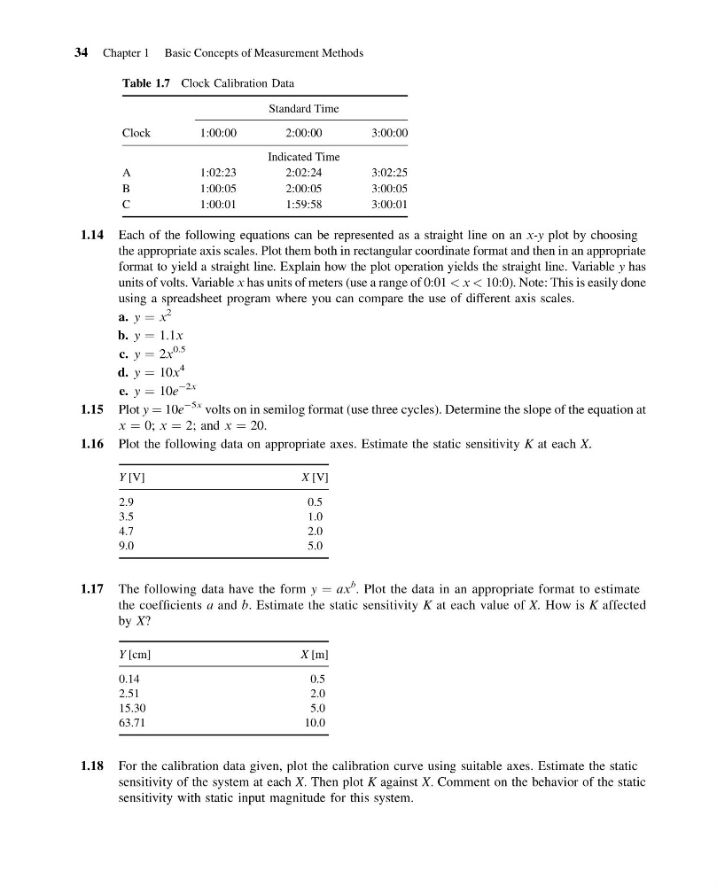
Table 1.7 Clock Calibration Data
Standard Time
Clock
1:00:00
2:00:00
3:00:00
Indicated Time
A
1:02:23
2:02:24
3:02:25
B
1:00:05
2:00:05
3:00:05
C
1:00:01
1:59:58
3:00:01
34 Chapter 1 Basic Concepts of Measurement Methods
15:40:39 Page 34
1.14 Each of the following equations can be represented as a straight line on an x-y plot by choosing
the appropriate axis scales. Plot them both in rectangular coordinate format and then in an appropriate
format to yield a straight line. Explain how the plot operation yields the straight line. Variable y has
units of volts. Variable x has units of meters (use a range of 0:01 < x < 10:0). Note: This is easily done
using a spreadsheet program where you can compare the use of different axis scales.
a. y ¼ x
2
b. y ¼ 1.1x
c. y ¼ 2x
0.5
d. y ¼ 10x
4
e. y ¼ 10e
À2x
1.15 Plot y ¼ 10e
À5x volts on in semilog format (use three cycles). Determine the slope of the equation at
x ¼ 0; x ¼ 2; and x ¼ 20.
1.16 Plot the following data on appropriate axes. Estimate the static sensitivity K at each X.
Y [V]
X [V]
2.9
0.5
3.5
1.0
4.7
2.0
9.0
5.0
1.17 The following data have the form y ¼ ax
b . Plot the data in an appropriate format to estimate
the coefficients a and b. Estimate the static sensitivity K at each value of X. How is K affected
by X?
Y [cm]
X [m]
0.14
0.5
2.51
2.0
15.30
5.0
63.71
10.0
1.18 For the calibration data given, plot the calibration curve using suitable axes. Estimate the static
sensitivity of the system at each X. Then plot K against X. Comment on the behavior of the static
sensitivity with static input magnitude for this system.
Table 1.7 Clock Calibration Data
Standard Time
Clock
1:00:00
2:00:00
3:00:00
Indicated Time
A
1:02:23
2:02:24
3:02:25
B
1:00:05
2:00:05
3:00:05
C
1:00:01
1:59:58
3:00:01
34 Chapter 1 Basic Concepts of Measurement Methods