

E1C09 09/14/2010
15:4:54 Page 394
A reciprocating piston within a cylinder can generate a sinusoidal variation in pressure for
frequency-response calibration. The piston can be driven by a variable speed motor and its displacement measured by a fast-responding transducer, such as an LVDT (see Chapter 12). Under
properly controlled conditions (Ex. 1.2), the actual pressure variation can be estimated from the
piston displacement. Other techniques include an encased loudspeaker or an acoustically resonant
enclosure, which serves as a frequency driver instead of a piston, or using an oscillating flow control
valve to vary system pressure with time (6).
Example 9.6
A surgical pressure transducer is attached to a stiff-walled catheter and a small balloon is attached at its
other end. The catheter is filled with saline using a small syringe to pressurize the system to 80 mm Hg.
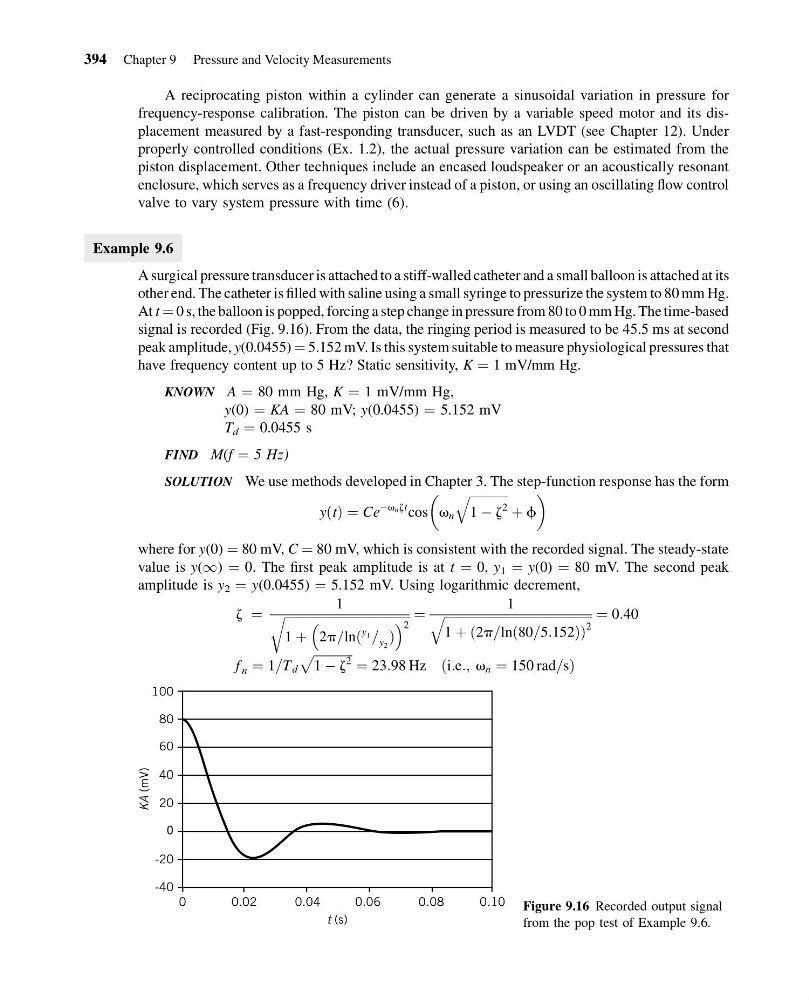
At t ¼ 0 s, the balloon is popped, forcing a step change in pressure from 80 to 0 mm Hg. The time-based
signal is recorded (Fig. 9.16). From the data, the ringing period is measured to be 45.5 ms at second
peak amplitude, y(0.0455) ¼ 5.152 mV. Is this system suitable to measure physiological pressures that
have frequency content up to 5 Hz? Static sensitivity, K ¼ 1 mV/mm Hg.
KNOWN A ¼ 80 mm Hg, K ¼ 1 mV/mm Hg,
y(0) ¼ KA ¼ 80 mV; y(0.0455) ¼ 5.152 mV
T d ¼ 0.0455 s
FIND M(f ¼ 5 Hz)
SOLUTION We use methods developed in Chapter 3. The step-function response has the form
yðtÞ ¼ Ce
Àv n zt cos
v n
ffiffiffiffiffiffiffiffiffiffiffiffi ffi
1 À z
2
q
þ f
where for y(0) ¼ 80 mV, C ¼ 80 mV, which is consistent with the recorded signal. The steady-state
value is y(1) ¼ 0. The first peak amplitude is at t ¼ 0, y 1 ¼ y(0) ¼ 80 mV. The second peak
amplitude is y 2 ¼ y(0.0455) ¼ 5.152 mV. Using logarithmic decrement,
z ¼
1
ffiffiffiffiffiffiffiffiffiffiffiffiffiffiffiffiffiffiffiffiffiffiffiffiffiffiffiffiffiffiffiffiffiffiffiffiffiffiffiffi ffi
1 þ 2p=lnð
y 1 = y 2 Þ
2
r
¼
1
ffiffiffiffiffiffiffiffiffiffiffiffiffiffiffiffiffiffiffiffiffiffiffiffiffiffiffiffiffiffiffiffiffiffiffiffiffiffiffiffiffiffiffiffiffiffiffi ffi
1 þ 2p=lnð80=5:152Þ
ð
Þ
2
q
¼ 0:40
f n ¼ 1=T d
ffiffiffiffiffiffiffiffiffiffiffiffi ffi
1 À z
2
p
¼ 23:98 Hz ði:e:; v n ¼ 150 rad=sÞ
100
80
60
40
KA (mV)
20
0
-20
-40
t (s)
0
0.02
0.04
0.06
0.08
0.10 Figure 9.16 Recorded output signal
from the pop test of Example 9.6.
394 Chapter 9 Pressure and Velocity Measurements
15:4:54 Page 394
A reciprocating piston within a cylinder can generate a sinusoidal variation in pressure for
frequency-response calibration. The piston can be driven by a variable speed motor and its displacement measured by a fast-responding transducer, such as an LVDT (see Chapter 12). Under
properly controlled conditions (Ex. 1.2), the actual pressure variation can be estimated from the
piston displacement. Other techniques include an encased loudspeaker or an acoustically resonant
enclosure, which serves as a frequency driver instead of a piston, or using an oscillating flow control
valve to vary system pressure with time (6).
Example 9.6
A surgical pressure transducer is attached to a stiff-walled catheter and a small balloon is attached at its
other end. The catheter is filled with saline using a small syringe to pressurize the system to 80 mm Hg.
At t ¼ 0 s, the balloon is popped, forcing a step change in pressure from 80 to 0 mm Hg. The time-based
signal is recorded (Fig. 9.16). From the data, the ringing period is measured to be 45.5 ms at second
peak amplitude, y(0.0455) ¼ 5.152 mV. Is this system suitable to measure physiological pressures that
have frequency content up to 5 Hz? Static sensitivity, K ¼ 1 mV/mm Hg.
KNOWN A ¼ 80 mm Hg, K ¼ 1 mV/mm Hg,
y(0) ¼ KA ¼ 80 mV; y(0.0455) ¼ 5.152 mV
T d ¼ 0.0455 s
FIND M(f ¼ 5 Hz)
SOLUTION We use methods developed in Chapter 3. The step-function response has the form
yðtÞ ¼ Ce
Àv n zt cos
v n
ffiffiffiffiffiffiffiffiffiffiffiffi ffi
1 À z
2
q
þ f
where for y(0) ¼ 80 mV, C ¼ 80 mV, which is consistent with the recorded signal. The steady-state
value is y(1) ¼ 0. The first peak amplitude is at t ¼ 0, y 1 ¼ y(0) ¼ 80 mV. The second peak
amplitude is y 2 ¼ y(0.0455) ¼ 5.152 mV. Using logarithmic decrement,
z ¼
1
ffiffiffiffiffiffiffiffiffiffiffiffiffiffiffiffiffiffiffiffiffiffiffiffiffiffiffiffiffiffiffiffiffiffiffiffiffiffiffiffi ffi
1 þ 2p=lnð
y 1 = y 2 Þ
2
r
¼
1
ffiffiffiffiffiffiffiffiffiffiffiffiffiffiffiffiffiffiffiffiffiffiffiffiffiffiffiffiffiffiffiffiffiffiffiffiffiffiffiffiffiffiffiffiffiffiffi ffi
1 þ 2p=lnð80=5:152Þ
ð
Þ
2
q
¼ 0:40
f n ¼ 1=T d
ffiffiffiffiffiffiffiffiffiffiffiffi ffi
1 À z
2
p
¼ 23:98 Hz ði:e:; v n ¼ 150 rad=sÞ
100
80
60
40
KA (mV)
20
0
-20
-40
t (s)
0
0.02
0.04
0.06
0.08
0.10 Figure 9.16 Recorded output signal
from the pop test of Example 9.6.
394 Chapter 9 Pressure and Velocity Measurements