

E1C01 09/14/2010
15:40:35 Page 21
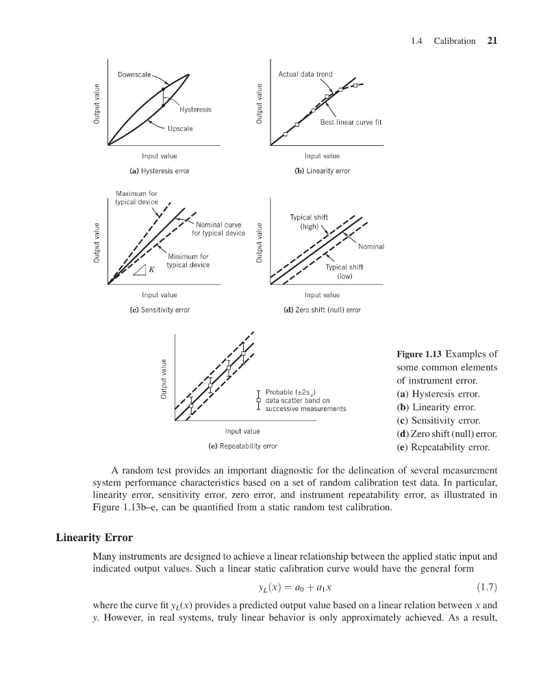
A random test provides an important diagnostic for the delineation of several measurement
system performance characteristics based on a set of random calibration test data. In particular,
linearity error, sensitivity error, zero error, and instrument repeatability error, as illustrated in
Figure 1.13b–e, can be quantified from a static random test calibration.
Linearity Error
Many instruments are designed to achieve a linear relationship between the applied static input and
indicated output values. Such a linear static calibration curve would have the general form
y L x
ð Þ ¼ a 0 þ a 1 x
ð1:7Þ
where the curve fit y L (x) provides a predicted output value based on a linear relation between x and
y. However, in real systems, truly linear behavior is only approximately achieved. As a result,
Input value
Maximum for
typical device
Nominal curve
for typical device
Minimum for
typical device
K
(a) Hysteresis error
Output value
Input value
(b) Linearity error
Output value
Input value
(c) Sensitivity error
Output value
Input value
(e) Repeatability error
Output value
Input value
(d) Zero shift (null) error
Output value
Upscale
Hysteresis
Best linear curve fit
Typical shift
(high)
Typical shift
(low)
Nominal
Actual data trend
Downscale
Probable (±2s x )
data scatter band on
successive measurements
Figure 1.13 Examples of
some common elements
of instrument error.
(a) Hysteresis error.
(b) Linearity error.
(c) Sensitivity error.
(d) Zero shift (null) error.
(e) Repeatability error.
1.4 Calibration 21
15:40:35 Page 21
A random test provides an important diagnostic for the delineation of several measurement
system performance characteristics based on a set of random calibration test data. In particular,
linearity error, sensitivity error, zero error, and instrument repeatability error, as illustrated in
Figure 1.13b–e, can be quantified from a static random test calibration.
Linearity Error
Many instruments are designed to achieve a linear relationship between the applied static input and
indicated output values. Such a linear static calibration curve would have the general form
y L x
ð Þ ¼ a 0 þ a 1 x
ð1:7Þ
where the curve fit y L (x) provides a predicted output value based on a linear relation between x and
y. However, in real systems, truly linear behavior is only approximately achieved. As a result,
Input value
Maximum for
typical device
Nominal curve
for typical device
Minimum for
typical device
K
(a) Hysteresis error
Output value
Input value
(b) Linearity error
Output value
Input value
(c) Sensitivity error
Output value
Input value
(e) Repeatability error
Output value
Input value
(d) Zero shift (null) error
Output value
Upscale
Hysteresis
Best linear curve fit
Typical shift
(high)
Typical shift
(low)
Nominal
Actual data trend
Downscale
Probable (±2s x )
data scatter band on
successive measurements
Figure 1.13 Examples of
some common elements
of instrument error.
(a) Hysteresis error.
(b) Linearity error.
(c) Sensitivity error.
(d) Zero shift (null) error.
(e) Repeatability error.
1.4 Calibration 21