

E1C07 09/14/2010
14:43:48 Page 262
second) or sample rate (in Hz) of
f s ¼ 1=dt
ð7:1Þ
For this discussion, we assume that the signal measurement occurs at a constant sample rate.
For each measurement, the amplitude of the sine wave is converted into a number. For comparison,
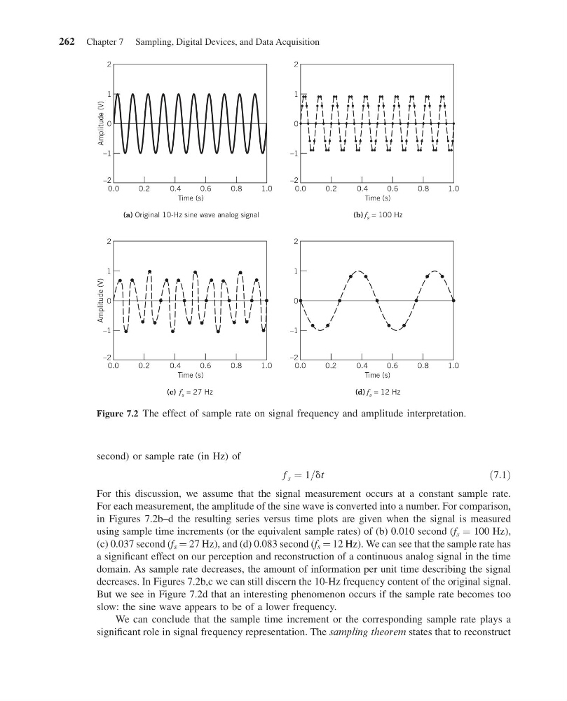
in Figures 7.2b–d the resulting series versus time plots are given when the signal is measured
using sample time increments (or the equivalent sample rates) of (b) 0.010 second (f s ¼ 100 Hz),
(c) 0.037 second (f s ¼ 27 Hz), and (d) 0.083 second (f s ¼ 12 Hz). We can see that the sample rate has
a significant effect on our perception and reconstruction of a continuous analog signal in the time
domain. As sample rate decreases, the amount of information per unit time describing the signal
decreases. In Figures 7.2b,c we can still discern the 10-Hz frequency content of the original signal.
But we see in Figure 7.2d that an interesting phenomenon occurs if the sample rate becomes too
slow: the sine wave appears to be of a lower frequency.
We can conclude that the sample time increment or the corresponding sample rate plays a
significant role in signal frequency representation. The sampling theorem states that to reconstruct
1.0
0.8
0.6
0.4
0.2
0.0
Time (s)
(c) f = 27 Hz
s
Amplitude (V)
–2
–1
0
1
2
1.0
0.8
0.6
0.4
0.2
0.0
Time (s)
(a) Original 10-Hz sine wave analog signal
Amplitude (V)
–2
–1
1
2
1.0
0.8
0.6
0.4
0.2
0.0
Time (s)
(d) f = 12 Hz
s
–2
–1
0
1
2
1.0
0.8
0.6
0.4
0.2
0.0
Time (s)
(b) f = 100 Hz
s
–2
–1
0
1
2
0
Figure 7.2 The effect of sample rate on signal frequency and amplitude interpretation.
262 Chapter 7 Sampling, Digital Devices, and Data Acquisition
14:43:48 Page 262
second) or sample rate (in Hz) of
f s ¼ 1=dt
ð7:1Þ
For this discussion, we assume that the signal measurement occurs at a constant sample rate.
For each measurement, the amplitude of the sine wave is converted into a number. For comparison,
in Figures 7.2b–d the resulting series versus time plots are given when the signal is measured
using sample time increments (or the equivalent sample rates) of (b) 0.010 second (f s ¼ 100 Hz),
(c) 0.037 second (f s ¼ 27 Hz), and (d) 0.083 second (f s ¼ 12 Hz). We can see that the sample rate has
a significant effect on our perception and reconstruction of a continuous analog signal in the time
domain. As sample rate decreases, the amount of information per unit time describing the signal
decreases. In Figures 7.2b,c we can still discern the 10-Hz frequency content of the original signal.
But we see in Figure 7.2d that an interesting phenomenon occurs if the sample rate becomes too
slow: the sine wave appears to be of a lower frequency.
We can conclude that the sample time increment or the corresponding sample rate plays a
significant role in signal frequency representation. The sampling theorem states that to reconstruct
1.0
0.8
0.6
0.4
0.2
0.0
Time (s)
(c) f = 27 Hz
s
Amplitude (V)
–2
–1
0
1
2
1.0
0.8
0.6
0.4
0.2
0.0
Time (s)
(a) Original 10-Hz sine wave analog signal
Amplitude (V)
–2
–1
1
2
1.0
0.8
0.6
0.4
0.2
0.0
Time (s)
(d) f = 12 Hz
s
–2
–1
0
1
2
1.0
0.8
0.6
0.4
0.2
0.0
Time (s)
(b) f = 100 Hz
s
–2
–1
0
1
2
0
Figure 7.2 The effect of sample rate on signal frequency and amplitude interpretation.
262 Chapter 7 Sampling, Digital Devices, and Data Acquisition