

E1C05 09/14/2010
14:36:26 Page 174
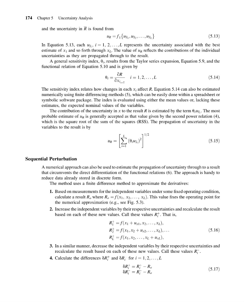
and the uncertainty in R is found from
u R ¼ f 1 u x 1 ; u x 2 ; . . . ; u x L
È
É
ð5:13Þ
In Equation 5.13, each u x i ; i ¼ 1; 2; . . . ; L represents the uncertainty associated with the best
estimate of x 1 and so forth through x L . The value of u R reflects the contributions of the individual
uncertainties as they are propagated through to the result.
A general sensitivity index, u i , results from the Taylor series expansion, Equation 5.9, and the
functional relation of Equation 5.10 and is given by
u i ¼
qR
qx i x¼x
i ¼ 1; 2; . . . ; L
ð5:14Þ
The sensitivity index relates how changes in each x i affect R. Equation 5.14 can also be estimated
numerically using finite differencing methods (5), which can be easily done within a spreadsheet or
symbolic software package. The index is evaluated using either the mean values or, lacking these
estimates, the expected nominal values of the variables.
The contribution of the uncertainty in x to the result R is estimated by the term u i u x i . The most
probable estimate of u R is generally accepted as that value given by the second power relation (4),
which is the square root of the sum of the squares (RSS). The propagation of uncertainty in the
variables to the result is by
u R ¼
X L
i¼1
ðu i u x i Þ
2
"
# 1=2
ð5:15Þ
Sequential Perturbation
A numerical approach can also be used to estimate the propagation of uncertainty through to a result
that circumvents the direct differentiation of the functional relations (6). The approach is handy to
reduce data already stored in discrete form.
The method uses a finite difference method to approximate the derivatives:
1. Based on measurements for the independent variables under some fixed operating condition,
calculate a result R o where R o ¼ f x 1 ; x 2 ; . . . ; x L
ð
Þ . This value fixes the operating point for
the numerical approximation (e.g., see Fig. 5.3).
2. Increase the independent variables by their respective uncertainties and recalculate the result
based on each of these new values. Call these values R
þ
i . That is,
R
þ
1 ¼ f x 1 þ u x1 ; x 2 ; . . . ; x L
ð
Þ ;
R
þ
2 ¼ f x 1 ; x 2 þ u x2 ; . . . ; x L
ð
Þ ; . . .
R
þ
L ¼ f x 1 ; x 2 ; . . . ; x L þ u xL
ð
Þ ;
ð5:16Þ
3. In a similar manner, decrease the independent variables by their respective uncertainties and
recalculate the result based on each of these new values. Call these values R
À
i .
4. Calculate the differences dR
þ
i and dR
À
i for i ¼ 1; 2; . . . ; L
dR
þ
i ¼ R
þ
i À R o
dR
À
i ¼ R
À
i À R o
ð5:17Þ
174 Chapter 5 Uncertainty Analysis
14:36:26 Page 174
and the uncertainty in R is found from
u R ¼ f 1 u x 1 ; u x 2 ; . . . ; u x L
È
É
ð5:13Þ
In Equation 5.13, each u x i ; i ¼ 1; 2; . . . ; L represents the uncertainty associated with the best
estimate of x 1 and so forth through x L . The value of u R reflects the contributions of the individual
uncertainties as they are propagated through to the result.
A general sensitivity index, u i , results from the Taylor series expansion, Equation 5.9, and the
functional relation of Equation 5.10 and is given by
u i ¼
qR
qx i x¼x
i ¼ 1; 2; . . . ; L
ð5:14Þ
The sensitivity index relates how changes in each x i affect R. Equation 5.14 can also be estimated
numerically using finite differencing methods (5), which can be easily done within a spreadsheet or
symbolic software package. The index is evaluated using either the mean values or, lacking these
estimates, the expected nominal values of the variables.
The contribution of the uncertainty in x to the result R is estimated by the term u i u x i . The most
probable estimate of u R is generally accepted as that value given by the second power relation (4),
which is the square root of the sum of the squares (RSS). The propagation of uncertainty in the
variables to the result is by
u R ¼
X L
i¼1
ðu i u x i Þ
2
"
# 1=2
ð5:15Þ
Sequential Perturbation
A numerical approach can also be used to estimate the propagation of uncertainty through to a result
that circumvents the direct differentiation of the functional relations (6). The approach is handy to
reduce data already stored in discrete form.
The method uses a finite difference method to approximate the derivatives:
1. Based on measurements for the independent variables under some fixed operating condition,
calculate a result R o where R o ¼ f x 1 ; x 2 ; . . . ; x L
ð
Þ . This value fixes the operating point for
the numerical approximation (e.g., see Fig. 5.3).
2. Increase the independent variables by their respective uncertainties and recalculate the result
based on each of these new values. Call these values R
þ
i . That is,
R
þ
1 ¼ f x 1 þ u x1 ; x 2 ; . . . ; x L
ð
Þ ;
R
þ
2 ¼ f x 1 ; x 2 þ u x2 ; . . . ; x L
ð
Þ ; . . .
R
þ
L ¼ f x 1 ; x 2 ; . . . ; x L þ u xL
ð
Þ ;
ð5:16Þ
3. In a similar manner, decrease the independent variables by their respective uncertainties and
recalculate the result based on each of these new values. Call these values R
À
i .
4. Calculate the differences dR
þ
i and dR
À
i for i ¼ 1; 2; . . . ; L
dR
þ
i ¼ R
þ
i À R o
dR
À
i ¼ R
À
i À R o
ð5:17Þ
174 Chapter 5 Uncertainty Analysis