

E1C05 09/14/2010
14:36:26 Page 172
with degrees of freedom n ¼ N À 1 and assuming the errors are normally distributed.
5 The interval
has a confidence level of one standard deviation, equivalent to a probability of 68% for a population
of x having a normal distribution. The random uncertainty at a desired confidence level is defined by
the interval Æt v;P s x , where t is found from Table 4.4.
5.6 UNCERTAINTY ANALYSIS: ERROR PROPAGATION
Suppose we want to determine how long it would take to fill a swimming pool from a garden hose.
One way is to measure the time required to fill a bucket of known volume to estimate the flow rate
from the garden hose. Armed with a measurement of the volume of the pool, we can calculate the
time to fill the pool. Clearly, small errors in estimating the flow rate from the garden hose would
translate into large differences in the time required to fill the pool! Here we are using measured
values, the flow rate and volume, to estimate a result, the time required to fill the pool.
Very often in engineering, results are determined through a functional relationship with measured
values. For example, we just calculated a flow rate above by measuring time, t, and bucket volume, 8,
since Q ¼ f ðt; 8Þ ¼ 8=t. But how do uncertainties in either measured quantity contribute to uncertainty
in flow rate? Is the uncertainty in Q more sensitive to uncertainty in volume or in time? More generally,
how are uncertainties in variables propagated to a calculated result? We now explore these questions.
Propagation of Error
A general relationship between some dependent variable y and a measured variable x, that is,
y ¼ f ðxÞ, is illustrated in Figure 5.3. Now suppose we measure x a number of times at some
operating condition so as to establish its sample mean value and the uncertainty due to random error
in this mean value, t n;P s x , which for convenience we write simply as ts x . This implies that,
neglecting other random and systematic errors, the true value for x lies somewhere within the
interval x Æ ts x . It is reasonable to assume that the true value of y, which is determined from the
measured values of x, falls within the interval defined by
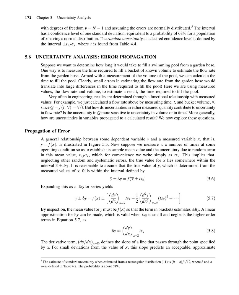
y Æ dy ¼ f x Æ ts x
ð
Þ
ð5:6Þ
Expanding this as a Taylor series yields
y Æ dy ¼ f x
ð Þ Æ
dy
dx
x¼x
ts x þ
1
2
d
2
y
dx 2
x¼x
ðts x Þ
2 þ Á Á Á
!
ð5:7Þ
By inspection, the mean value for y must be f x
ð Þ so that the term in brackets estimates Ædy. A linear
approximation for dy can be made, which is valid when ts x is small and neglects the higher order
terms in Equation 5.7, as
dy %
dy
dx
x¼x
ts x
ð5:8Þ
The derivative term, dy=dx
ð
Þ x¼x , defines the slope of a line that passes through the point specified
by x. For small deviations from the value of x, this slope predicts an acceptable, approximate
5 The estimate of standard uncertainty when estimated from a rectangular distribution (11) is ðb À aÞ=
ffiffiffiffiffi
12
p
, where b and a
were defined in Table 4.2. The probability is about 58%.
172 Chapter 5 Uncertainty Analysis
14:36:26 Page 172
with degrees of freedom n ¼ N À 1 and assuming the errors are normally distributed.
5 The interval
has a confidence level of one standard deviation, equivalent to a probability of 68% for a population
of x having a normal distribution. The random uncertainty at a desired confidence level is defined by
the interval Æt v;P s x , where t is found from Table 4.4.
5.6 UNCERTAINTY ANALYSIS: ERROR PROPAGATION
Suppose we want to determine how long it would take to fill a swimming pool from a garden hose.
One way is to measure the time required to fill a bucket of known volume to estimate the flow rate
from the garden hose. Armed with a measurement of the volume of the pool, we can calculate the
time to fill the pool. Clearly, small errors in estimating the flow rate from the garden hose would
translate into large differences in the time required to fill the pool! Here we are using measured
values, the flow rate and volume, to estimate a result, the time required to fill the pool.
Very often in engineering, results are determined through a functional relationship with measured
values. For example, we just calculated a flow rate above by measuring time, t, and bucket volume, 8,
since Q ¼ f ðt; 8Þ ¼ 8=t. But how do uncertainties in either measured quantity contribute to uncertainty
in flow rate? Is the uncertainty in Q more sensitive to uncertainty in volume or in time? More generally,
how are uncertainties in variables propagated to a calculated result? We now explore these questions.
Propagation of Error
A general relationship between some dependent variable y and a measured variable x, that is,
y ¼ f ðxÞ, is illustrated in Figure 5.3. Now suppose we measure x a number of times at some
operating condition so as to establish its sample mean value and the uncertainty due to random error
in this mean value, t n;P s x , which for convenience we write simply as ts x . This implies that,
neglecting other random and systematic errors, the true value for x lies somewhere within the
interval x Æ ts x . It is reasonable to assume that the true value of y, which is determined from the
measured values of x, falls within the interval defined by
y Æ dy ¼ f x Æ ts x
ð
Þ
ð5:6Þ
Expanding this as a Taylor series yields
y Æ dy ¼ f x
ð Þ Æ
dy
dx
x¼x
ts x þ
1
2
d
2
y
dx 2
x¼x
ðts x Þ
2 þ Á Á Á
!
ð5:7Þ
By inspection, the mean value for y must be f x
ð Þ so that the term in brackets estimates Ædy. A linear
approximation for dy can be made, which is valid when ts x is small and neglects the higher order
terms in Equation 5.7, as
dy %
dy
dx
x¼x
ts x
ð5:8Þ
The derivative term, dy=dx
ð
Þ x¼x , defines the slope of a line that passes through the point specified
by x. For small deviations from the value of x, this slope predicts an acceptable, approximate
5 The estimate of standard uncertainty when estimated from a rectangular distribution (11) is ðb À aÞ=
ffiffiffiffiffi
12
p
, where b and a
were defined in Table 4.2. The probability is about 58%.
172 Chapter 5 Uncertainty Analysis