

E1C04 09/14/2010
14:7:43 Page 140
sampling is made under the new operating conditions. This is a common procedure used to document
the relationship between the measured variable and an independent process variable. We can use
regression analysis to establish a functional relationship between the dependent variable and the
independent variable. This discussion pertains directly to polynomial curve fits. More information on
regression analysis, including multiple variable regression, can be found elsewhere (4, 6).
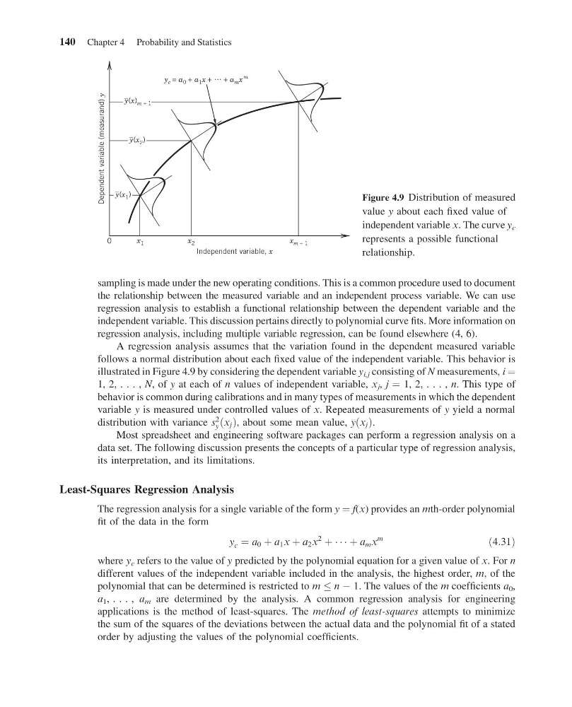
A regression analysis assumes that the variation found in the dependent measured variable
follows a normal distribution about each fixed value of the independent variable. This behavior is
illustrated in Figure 4.9 by considering the dependent variable y i,j consisting of N measurements, i ¼
1, 2, . . . , N, of y at each of n values of independent variable, x j , j ¼ 1, 2, . . . , n. This type of
behavior is common during calibrations and in many types of measurements in which the dependent
variable y is measured under controlled values of x. Repeated measurements of y yield a normal
distribution with variance s
2
y ðx j Þ, about some mean value, yðx j Þ.
Most spreadsheet and engineering software packages can perform a regression analysis on a
data set. The following discussion presents the concepts of a particular type of regression analysis,
its interpretation, and its limitations.
Least-Squares Regression Analysis
The regression analysis for a single variable of the form y ¼ f(x) provides an mth-order polynomial
fit of the data in the form
y c ¼ a 0 þ a 1 x þ a 2 x
2
þ Á Á Á þ a m x
m
ð4:31Þ
where y c refers to the value of y predicted by the polynomial equation for a given value of x. For n
different values of the independent variable included in the analysis, the highest order, m, of the
polynomial that can be determined is restricted to m n À 1. The values of the m coefficients a 0 ,
a 1 , . . . , a m are determined by the analysis. A common regression analysis for engineering
applications is the method of least-squares. The method of least-squares attempts to minimize
the sum of the squares of the deviations between the actual data and the polynomial fit of a stated
order by adjusting the values of the polynomial coefficients.
x 1
x 2
x m + 1
Independent variable, x
Dependent variable (measurand)
y
y c = a 0 + a 1 x +
+ a m x
m
y(x 2 )
–
y(x 1 )
–
y(x) m + 1
0
–
Figure 4.9 Distribution of measured
value y about each fixed value of
independent variable x. The curve y c
represents a possible functional
relationship.
140 Chapter 4 Probability and Statistics
14:7:43 Page 140
sampling is made under the new operating conditions. This is a common procedure used to document
the relationship between the measured variable and an independent process variable. We can use
regression analysis to establish a functional relationship between the dependent variable and the
independent variable. This discussion pertains directly to polynomial curve fits. More information on
regression analysis, including multiple variable regression, can be found elsewhere (4, 6).
A regression analysis assumes that the variation found in the dependent measured variable
follows a normal distribution about each fixed value of the independent variable. This behavior is
illustrated in Figure 4.9 by considering the dependent variable y i,j consisting of N measurements, i ¼
1, 2, . . . , N, of y at each of n values of independent variable, x j , j ¼ 1, 2, . . . , n. This type of
behavior is common during calibrations and in many types of measurements in which the dependent
variable y is measured under controlled values of x. Repeated measurements of y yield a normal
distribution with variance s
2
y ðx j Þ, about some mean value, yðx j Þ.
Most spreadsheet and engineering software packages can perform a regression analysis on a
data set. The following discussion presents the concepts of a particular type of regression analysis,
its interpretation, and its limitations.
Least-Squares Regression Analysis
The regression analysis for a single variable of the form y ¼ f(x) provides an mth-order polynomial
fit of the data in the form
y c ¼ a 0 þ a 1 x þ a 2 x
2
þ Á Á Á þ a m x
m
ð4:31Þ
where y c refers to the value of y predicted by the polynomial equation for a given value of x. For n
different values of the independent variable included in the analysis, the highest order, m, of the
polynomial that can be determined is restricted to m n À 1. The values of the m coefficients a 0 ,
a 1 , . . . , a m are determined by the analysis. A common regression analysis for engineering
applications is the method of least-squares. The method of least-squares attempts to minimize
the sum of the squares of the deviations between the actual data and the polynomial fit of a stated
order by adjusting the values of the polynomial coefficients.
x 1
x 2
x m + 1
Independent variable, x
Dependent variable (measurand)
y
y c = a 0 + a 1 x +
+ a m x
m
y(x 2 )
–
y(x 1 )
–
y(x) m + 1
0
–
Figure 4.9 Distribution of measured
value y about each fixed value of
independent variable x. The curve y c
represents a possible functional
relationship.
140 Chapter 4 Probability and Statistics