

E1C04 09/14/2010
14:7:43 Page 139
FIND Apply the chi-squared test to the data set to test for normal distribution.
SOLUTION Figure 4.2 (Ex. 4.1) provides a histogram for the data of Table 4.1 giving the
values for n j for K ¼ 7 intervals. To evaluate the hypothesis, we must find the predicted number of
occurrences, n
0
j , for each of the seven intervals based on a normal distribution. To do this, substitute
x
0
¼ x and s ¼ s x and compute the probabilities based on the corresponding z values.
For example, consider the second interval (j ¼ 2). Using Table 4.3, the predicted probabilities
are
Pð0:75 x i 0:85Þ¼ Pð0:75 x i < x
0
Þ À Pð0:85 x i < x
0
Þ
¼ Pðz a Þ À Pðz b Þ
¼ Pð1:6875Þ À Pð1:0625Þ
¼ 0:454 À 0:356 ¼ 0:098
So for a normal distribution, we should expect the measured value to lie within the second interval
for 9.8% of the measurements. With
n
0
2 ¼ N Â Pð0:75 x i < 0:85Þ ¼ 20 Â 0:098 ¼ 1:96
that is, 1.96 occurrences are expected out of 20 measurements in this second interval. The actual
measured data set shows n 2 ¼ 1.
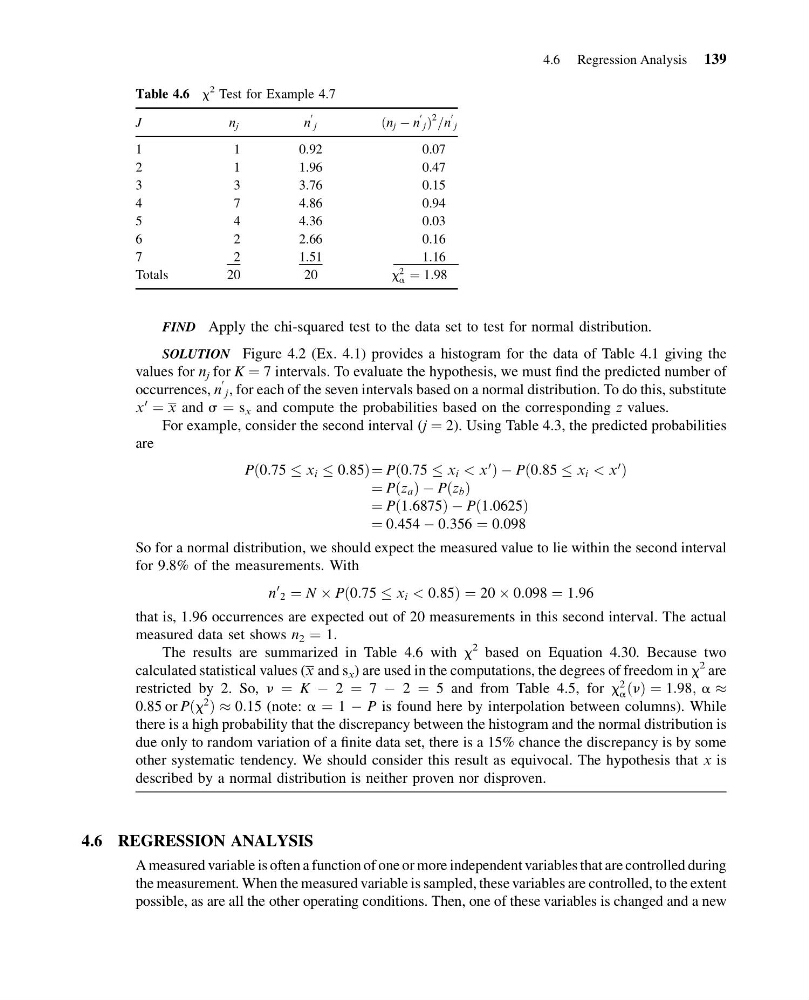
The results are summarized in Table 4.6 with x
2 based on Equation 4.30. Because two
calculated statistical values (x and s x ) are used in the computations, the degrees of freedom in x
2 are
restricted by 2. So, n ¼ K À 2 ¼ 7 À 2 ¼ 5 and from Table 4.5, for x
2
a ðnÞ ¼ 1:98; a %
0:85 or Pðx
2
Þ % 0:15 (note: a ¼ 1 À P is found here by interpolation between columns). While
there is a high probability that the discrepancy between the histogram and the normal distribution is
due only to random variation of a finite data set, there is a 15% chance the discrepancy is by some
other systematic tendency. We should consider this result as equivocal. The hypothesis that x is
described by a normal distribution is neither proven nor disproven.
4.6 REGRESSION ANALYSIS
A measured variable is often a function of one or more independent variables that are controlled during
the measurement. When the measured variable is sampled, these variables are controlled, to the extent
possible, as are all the other operating conditions. Then, one of these variables is changed and a new
Table 4.6 x
2 Test for Example 4.7
J
n j
n
0
j
ðn j À n
0
j Þ
2 =n
0
j
1
1
0.92
0.07
2
1
1.96
0.47
3
3
3.76
0.15
4
7
4.86
0.94
5
4
4.36
0.03
6
2
2.66
0.16
7
2
1.51
1.16
Totals
20
20
x
2
a ¼ 1:98
4.6 Regression Analysis 139
14:7:43 Page 139
FIND Apply the chi-squared test to the data set to test for normal distribution.
SOLUTION Figure 4.2 (Ex. 4.1) provides a histogram for the data of Table 4.1 giving the
values for n j for K ¼ 7 intervals. To evaluate the hypothesis, we must find the predicted number of
occurrences, n
0
j , for each of the seven intervals based on a normal distribution. To do this, substitute
x
0
¼ x and s ¼ s x and compute the probabilities based on the corresponding z values.
For example, consider the second interval (j ¼ 2). Using Table 4.3, the predicted probabilities
are
Pð0:75 x i 0:85Þ¼ Pð0:75 x i < x
0
Þ À Pð0:85 x i < x
0
Þ
¼ Pðz a Þ À Pðz b Þ
¼ Pð1:6875Þ À Pð1:0625Þ
¼ 0:454 À 0:356 ¼ 0:098
So for a normal distribution, we should expect the measured value to lie within the second interval
for 9.8% of the measurements. With
n
0
2 ¼ N Â Pð0:75 x i < 0:85Þ ¼ 20 Â 0:098 ¼ 1:96
that is, 1.96 occurrences are expected out of 20 measurements in this second interval. The actual
measured data set shows n 2 ¼ 1.
The results are summarized in Table 4.6 with x
2 based on Equation 4.30. Because two
calculated statistical values (x and s x ) are used in the computations, the degrees of freedom in x
2 are
restricted by 2. So, n ¼ K À 2 ¼ 7 À 2 ¼ 5 and from Table 4.5, for x
2
a ðnÞ ¼ 1:98; a %
0:85 or Pðx
2
Þ % 0:15 (note: a ¼ 1 À P is found here by interpolation between columns). While
there is a high probability that the discrepancy between the histogram and the normal distribution is
due only to random variation of a finite data set, there is a 15% chance the discrepancy is by some
other systematic tendency. We should consider this result as equivocal. The hypothesis that x is
described by a normal distribution is neither proven nor disproven.
4.6 REGRESSION ANALYSIS
A measured variable is often a function of one or more independent variables that are controlled during
the measurement. When the measured variable is sampled, these variables are controlled, to the extent
possible, as are all the other operating conditions. Then, one of these variables is changed and a new
Table 4.6 x
2 Test for Example 4.7
J
n j
n
0
j
ðn j À n
0
j Þ
2 =n
0
j
1
1
0.92
0.07
2
1
1.96
0.47
3
3
3.76
0.15
4
7
4.86
0.94
5
4
4.36
0.03
6
2
2.66
0.16
7
2
1.51
1.16
Totals
20
20
x
2
a ¼ 1:98
4.6 Regression Analysis 139