

E1C03 09/14/2010
15:24:54 Page 103
v (rad/s)
M(v)
F(v) [
]
500
1.00
À3.3
2,600
1.04
À18.2
3,500
1.07
À25.6
6,155
1.15
À54.7
7,540
1.11
À73.9
8,706
1.00
À90.0
50,000
0.05
À170.2
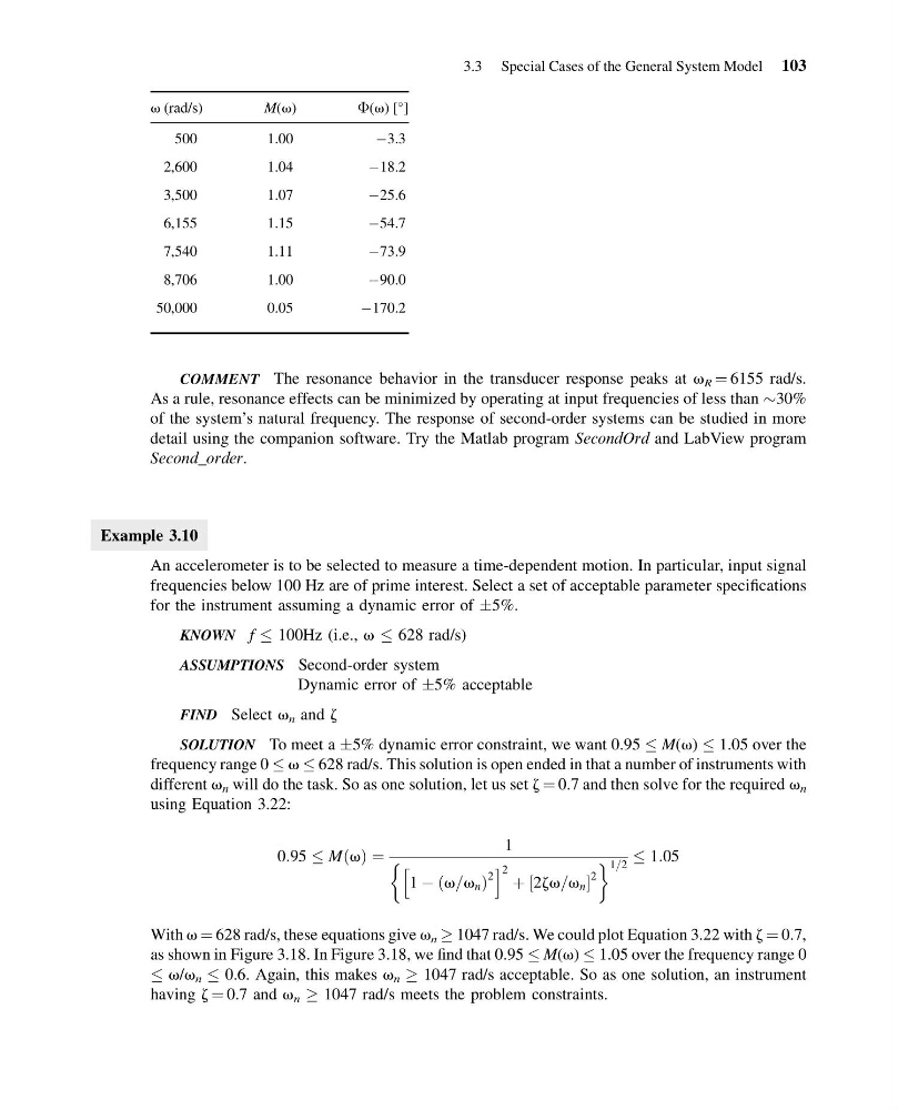
COMMENT The resonance behavior in the transducer response peaks at v R ¼ 6155 rad/s.
As a rule, resonance effects can be minimized by operating at input frequencies of less than $30%
of the system’s natural frequency. The response of second-order systems can be studied in more
detail using the companion software. Try the Matlab program SecondOrd and LabView program
Second_order.
Example 3.10
An accelerometer is to be selected to measure a time-dependent motion. In particular, input signal
frequencies below 100 Hz are of prime interest. Select a set of acceptable parameter specifications
for the instrument assuming a dynamic error of Æ5%.
KNOWN f 100Hz (i.e., v 628 rad/s)
ASSUMPTIONS Second-order system
Dynamic error of Æ5% acceptable
FIND Select v n and z
SOLUTION To meet a Æ5% dynamic error constraint, we want 0.95 M(v) 1.05 over the
frequency range 0 v 628 rad/s. This solution is open ended in that a number of instruments with
different v n will do the task. So as one solution, let us set z ¼ 0.7 and then solve for the required v n
using Equation 3.22:
0:95 M v
ð Þ ¼
1
1 À v=v n
ð
Þ
2
h
i 2 þ 2zv=v n
½
2
&
' 1=2 1:05
With v ¼ 628 rad/s, these equations give v n ! 1047 rad/s. We could plot Equation 3.22 with z ¼ 0.7,
as shown in Figure 3.18. In Figure 3.18, we find that 0.95 M(v) 1.05 over the frequency range 0
v/v n 0.6. Again, this makes v n ! 1047 rad/s acceptable. So as one solution, an instrument
having z ¼ 0.7 and v n ! 1047 rad/s meets the problem constraints.
3.3 Special Cases of the General System Model 103
15:24:54 Page 103
v (rad/s)
M(v)
F(v) [
]
500
1.00
À3.3
2,600
1.04
À18.2
3,500
1.07
À25.6
6,155
1.15
À54.7
7,540
1.11
À73.9
8,706
1.00
À90.0
50,000
0.05
À170.2
COMMENT The resonance behavior in the transducer response peaks at v R ¼ 6155 rad/s.
As a rule, resonance effects can be minimized by operating at input frequencies of less than $30%
of the system’s natural frequency. The response of second-order systems can be studied in more
detail using the companion software. Try the Matlab program SecondOrd and LabView program
Second_order.
Example 3.10
An accelerometer is to be selected to measure a time-dependent motion. In particular, input signal
frequencies below 100 Hz are of prime interest. Select a set of acceptable parameter specifications
for the instrument assuming a dynamic error of Æ5%.
KNOWN f 100Hz (i.e., v 628 rad/s)
ASSUMPTIONS Second-order system
Dynamic error of Æ5% acceptable
FIND Select v n and z
SOLUTION To meet a Æ5% dynamic error constraint, we want 0.95 M(v) 1.05 over the
frequency range 0 v 628 rad/s. This solution is open ended in that a number of instruments with
different v n will do the task. So as one solution, let us set z ¼ 0.7 and then solve for the required v n
using Equation 3.22:
0:95 M v
ð Þ ¼
1
1 À v=v n
ð
Þ
2
h
i 2 þ 2zv=v n
½
2
&
' 1=2 1:05
With v ¼ 628 rad/s, these equations give v n ! 1047 rad/s. We could plot Equation 3.22 with z ¼ 0.7,
as shown in Figure 3.18. In Figure 3.18, we find that 0.95 M(v) 1.05 over the frequency range 0
v/v n 0.6. Again, this makes v n ! 1047 rad/s acceptable. So as one solution, an instrument
having z ¼ 0.7 and v n ! 1047 rad/s meets the problem constraints.
3.3 Special Cases of the General System Model 103