

E1C03 09/14/2010
15:24:52 Page 88
In practice, it is best to record that response from t ¼ 0 until steady response is achieved. The data
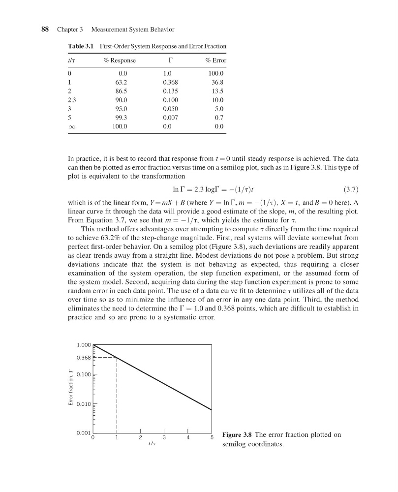
can then be plotted as error fraction versus time on a semilog plot, such as in Figure 3.8. This type of
plot is equivalent to the transformation
ln G ¼ 2:3 logG ¼ À 1=t
ð Þt
ð3:7Þ
which is of the linear form, Y ¼ mX þ B (where Y ¼ ln G, m ¼ Àð1=tÞ; X ¼ t; and B ¼ 0 here). A
linear curve fit through the data will provide a good estimate of the slope, m, of the resulting plot.
From Equation 3.7, we see that m ¼ À1=t, which yields the estimate for t.
This method offers advantages over attempting to compute t directly from the time required
to achieve 63.2% of the step-change magnitude. First, real systems will deviate somewhat from
perfect first-order behavior. On a semilog plot (Figure 3.8), such deviations are readily apparent
as clear trends away from a straight line. Modest deviations do not pose a problem. But strong
deviations indicate that the system is not behaving as expected, thus requiring a closer
examination of the system operation, the step function experiment, or the assumed form of
the system model. Second, acquiring data during the step function experiment is prone to some
random error in each data point. The use of a data curve fit to determine t utilizes all of the data
over time so as to minimize the influence of an error in any one data point. Third, the method
eliminates the need to determine the G ¼ 1:0 and 0.368 points, which are difficult to establish in
practice and so are prone to a systematic error.
Table 3.1 First-Order System Response and Error Fraction
t/t
% Response
G
% Error
0
0.0
1.0
100.0
1
63.2
0.368
36.8
2
86.5
0.135
13.5
2.3
90.0
0.100
10.0
3
95.0
0.050
5.0
5
99.3
0.007
0.7
1
100.0
0.0
0.0
0
0.001
0.010
0.100
1.000
0.368
1
2
3
4
5
Error fraction,
Γ
t/
Figure 3.8 The error fraction plotted on
semilog coordinates.
88 Chapter 3 Measurement System Behavior
15:24:52 Page 88
In practice, it is best to record that response from t ¼ 0 until steady response is achieved. The data
can then be plotted as error fraction versus time on a semilog plot, such as in Figure 3.8. This type of
plot is equivalent to the transformation
ln G ¼ 2:3 logG ¼ À 1=t
ð Þt
ð3:7Þ
which is of the linear form, Y ¼ mX þ B (where Y ¼ ln G, m ¼ Àð1=tÞ; X ¼ t; and B ¼ 0 here). A
linear curve fit through the data will provide a good estimate of the slope, m, of the resulting plot.
From Equation 3.7, we see that m ¼ À1=t, which yields the estimate for t.
This method offers advantages over attempting to compute t directly from the time required
to achieve 63.2% of the step-change magnitude. First, real systems will deviate somewhat from
perfect first-order behavior. On a semilog plot (Figure 3.8), such deviations are readily apparent
as clear trends away from a straight line. Modest deviations do not pose a problem. But strong
deviations indicate that the system is not behaving as expected, thus requiring a closer
examination of the system operation, the step function experiment, or the assumed form of
the system model. Second, acquiring data during the step function experiment is prone to some
random error in each data point. The use of a data curve fit to determine t utilizes all of the data
over time so as to minimize the influence of an error in any one data point. Third, the method
eliminates the need to determine the G ¼ 1:0 and 0.368 points, which are difficult to establish in
practice and so are prone to a systematic error.
Table 3.1 First-Order System Response and Error Fraction
t/t
% Response
G
% Error
0
0.0
1.0
100.0
1
63.2
0.368
36.8
2
86.5
0.135
13.5
2.3
90.0
0.100
10.0
3
95.0
0.050
5.0
5
99.3
0.007
0.7
1
100.0
0.0
0.0
0
0.001
0.010
0.100
1.000
0.368
1
2
3
4
5
Error fraction,
Γ
t/
Figure 3.8 The error fraction plotted on
semilog coordinates.
88 Chapter 3 Measurement System Behavior