

634
D Atomic and Molecular Term Symbols
For the example of a Si atom considered in §IV.2, where we found that the
(1s) 2 (2s) 2 (2p) 6 (3s) 2 (3p) 2 ground electronic configuration gave rise to three terms,
namely 1 S, 1 D, and 3 P , we see that J = L + S gives rise only to J = 0 for the 1 S
term, to J = 2 for the 1 D term, and to J = 2, 1, 0 for the 3 P term. The total number
of (J, M J )-states contained in the levels belonging to these terms is thus 15: 5 from
the 1 D 2 level, 1 from the 1 S 0 level, and 9 from the 3 P 2,1,0 levels. This is precisely
the number 6 · 5/2 of states for a (ns) 2 (np) 2 electronic configuration once the Pauli
Principle has been taken into account.
D.3 Term Symbols for Linear Molecules
The determination of term symbols for linear molecules proceeds similarly to what
we have just seen for atoms. We shall only draw the appropriate analogies here,
rather than go through a detailed derivation. The main idea is to use a new set of
designators: to this end, we note that we will use the correspondence
Atoms (roman letters) ←→ Molecules (Greek letters)
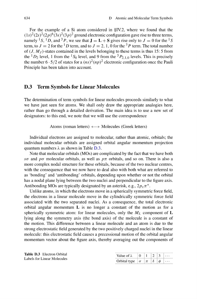
Individual electrons are assigned to molecular, rather than atomic, orbitals; the
individual molecular orbitals are assigned orbital angular momentum projection
quantum numbers λ as shown in Table D.3.
Note that molecular orbitals (MOs) are complicated by the fact that we have both
sσ and pσ molecular orbitals, as well as pπ orbitals, and so on. There is also a
more complex nodal structure for these orbitals, because of the two nuclear centres,
with the consequence that we now have to deal also with both what are referred to
as ‘bonding’ and ‘antibonding’ orbitals, depending upon whether or not the orbital
has a nodal plane lying between the two nuclei and perpendicular to the figure axis.
Antibonding MOs are typically designated by an asterisk, e.g., 2p x π ∗ .
Unlike atoms, in which the electrons move in a spherically symmetric force field,
the electrons in a linear molecule move in the cylindrically symmetric force field
associated with the two separated nuclei. As a consequence, the total electronic
orbital angular momentum L is no longer a constant of the motion as for a
spherically symmetric atom: for linear molecules, only the M L component of L
lying along the symmetry axis (the bond axis) of the molecule is a constant of
the motion. This difference between a linear molecule and an atom is due to the
strong electrostatic field generated by the two positively charged nuclei in the linear
molecule: this electrostatic field causes a precessional motion of the orbital angular
momentum vector about the figure axis, thereby averaging out the components of
Table D.3 Electron Orbital
Labels for Linear Molecules
Value of λ
0 1 2 3 · · ·
Orbital type σ π δ φ · · ·