

B.4 Jacobians
621
We may also write this equation in matrix format as
⎛
⎝
dy 1
dy 2
dy 3
⎞
⎠ =
⎛
⎝
f 1,x 1 f 1,x 2 f 1,x 3
f 2,x 1 f 2,x 2 f 2,x 3
f 3,x 1 f 3,x 2 f 3,x 3
⎞
⎠
⎛
⎝
dx 1
dx 2
dx 3
⎞
⎠ ,
(B.4.4)
or in the form
dy i =
3
j =1
f i,j dx j ,
i = 1, 2, 3 .
(B.4.5)
Notice that the set of Eqs. (B.4.2) describes a mapping of a domain of R 3 into R 3 ,
while Eqs. (B.4.3) describe a linear mapping which approximates the (in general
nonlinear) mapping (B.4.2) near a chosen point.
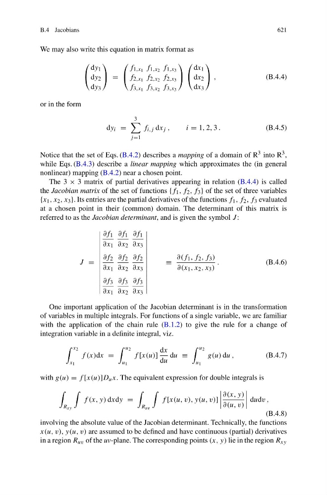
The 3 × 3 matrix of partial derivatives appearing in relation (B.4.4) is called
the Jacobian matrix of the set of functions {f 1 , f 2 , f 3 } of the set of three variables
{x 1 , x 2 , x 3 }. Its entries are the partial derivatives of the functions f 1 , f 2 , f 3 evaluated
at a chosen point in their (common) domain. The determinant of this matrix is
referred to as the Jacobian determinant, and is given the symbol J :
J =
∂f 1
∂x 1
∂f 1
∂x 2
∂f 1
∂x 3
∂f 2
∂x 1
∂f 2
∂x 2
∂f 2
∂x 3
∂f 3
∂x 1
∂f 3
∂x 2
∂f 3
∂x 3
≡
∂(f 1 , f 2 , f 3 )
∂(x 1 , x 2 , x 3 )
.
(B.4.6)
One important application of the Jacobian determinant is in the transformation
of variables in multiple integrals. For functions of a single variable, we are familiar
with the application of the chain rule (B.1.2) to give the rule for a change of
integration variable in a definite integral, viz.
x 2
x 1
f (x)dx =
u 2
u 1
f [x(u)]
dx
du
du ≡
u 2
u 1
g(u) du ,
(B.4.7)
with g(u) = f [x(u)]D u x. The equivalent expression for double integrals is
R xy
f (x, y) dxdy =
R uv
f [x(u, v), y(u, v)]
∂(x, y)
∂(u, v)
dudv ,
(B.4.8)
involving the absolute value of the Jacobian determinant. Technically, the functions
x(u, v), y(u, v) are assumed to be defined and have continuous (partial) derivatives
in a region R uv of the uv-plane. The corresponding points (x, y) lie in the region R xy