

10.6 Bose–Einstein Statistics
567
0
0.2
0.4
0.6
0.8
1
0
0.5
1
1.5
2
2.5
λ
g
n (λ)
n = 3/2
n = 5/2
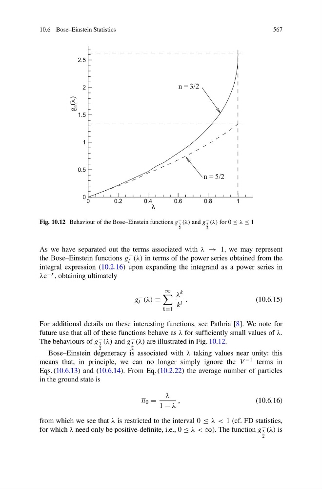
Fig. 10.12 Behaviour of the Bose–Einstein functions g
−
3
2
(λ) and g
−
5
2
(λ) for 0 ≤ λ ≤ 1
As we have separated out the terms associated with λ → 1, we may represent
the Bose–Einstein functions g
−
l (λ) in terms of the power series obtained from the
integral expression (10.2.16) upon expanding the integrand as a power series in
λe −x , obtaining ultimately
g
−
l (λ) ≡
∞
k=1
λ k
k l .
(10.6.15)
For additional details on these interesting functions, see Pathria [8]. We note for
future use that all of these functions behave as λ for sufficiently small values of λ.
The behaviours of g
−
3
2
(λ) and g
−
5
2
(λ) are illustrated in Fig. 10.12.
Bose–Einstein degeneracy is associated with λ taking values near unity: this
means that, in principle, we can no longer simply ignore the V −1 terms in
Eqs. (10.6.13) and (10.6.14). From Eq. (10.2.22) the average number of particles
in the ground state is
n 0 =
λ
1 − λ
,
(10.6.16)
from which we see that λ is restricted to the interval 0 ≤ λ < 1 (cf. FD statistics,
for which λ need only be positive-definite, i.e., 0 ≤ λ < ∞). The function g
−
3
2
(λ) is
567
0
0.2
0.4
0.6
0.8
1
0
0.5
1
1.5
2
2.5
λ
g
n (λ)
n = 3/2
n = 5/2
Fig. 10.12 Behaviour of the Bose–Einstein functions g
−
3
2
(λ) and g
−
5
2
(λ) for 0 ≤ λ ≤ 1
As we have separated out the terms associated with λ → 1, we may represent
the Bose–Einstein functions g
−
l (λ) in terms of the power series obtained from the
integral expression (10.2.16) upon expanding the integrand as a power series in
λe −x , obtaining ultimately
g
−
l (λ) ≡
∞
k=1
λ k
k l .
(10.6.15)
For additional details on these interesting functions, see Pathria [8]. We note for
future use that all of these functions behave as λ for sufficiently small values of λ.
The behaviours of g
−
3
2
(λ) and g
−
5
2
(λ) are illustrated in Fig. 10.12.
Bose–Einstein degeneracy is associated with λ taking values near unity: this
means that, in principle, we can no longer simply ignore the V −1 terms in
Eqs. (10.6.13) and (10.6.14). From Eq. (10.2.22) the average number of particles
in the ground state is
n 0 =
λ
1 − λ
,
(10.6.16)
from which we see that λ is restricted to the interval 0 ≤ λ < 1 (cf. FD statistics,
for which λ need only be positive-definite, i.e., 0 ≤ λ < ∞). The function g
−
3
2
(λ) is