

554
10 Quantum Statistics
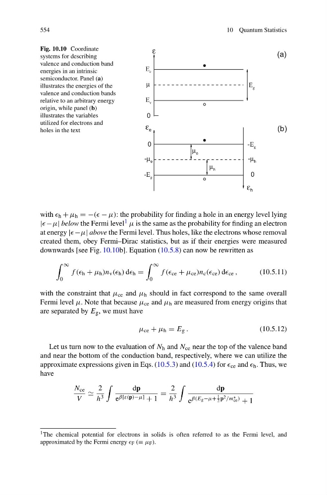
Fig. 10.10 Coordinate
systems for describing
valence and conduction band
energies in an intrinsic
semiconductor. Panel (a)
illustrates the energies of the
valence and conduction bands
relative to an arbitrary energy
origin, while panel (b)
illustrates the variables
utilized for electrons and
holes in the text
ε
E c
μ
E v
E g
0
(a)
ε e
μ e
-E g
-E g
0
0
μ h
ε h
-μ e
-μ h
(b)
with h + μ h = −(( − μ): the probability for finding a hole in an energy level lying
| −μ| below the Fermi level 1 μ is the same as the probability for finding an electron
at energy |−μ| above the Fermi level. Thus holes, like the electrons whose removal
created them, obey Fermi–Dirac statistics, but as if their energies were measured
downwards [see Fig. 10.10b]. Equation (10.5.8) can now be rewritten as
∞
0
f (( h + μ h )n v (( h ) d h =
∞
0
f (( ce + μ ce )n c (( ce ) d ce ,
(10.5.11)
with the constraint that μ ce and μ h should in fact correspond to the same overall
Fermi level μ. Note that because μ ce and μ h are measured from energy origins that
are separated by E g , we must have
μ ce + μ h = E g .
(10.5.12)
Let us turn now to the evaluation of N h and N ce near the top of the valence band
and near the bottom of the conduction band, respectively, where we can utilize the
approximate expressions given in Eqs. (10.5.3) and (10.5.4) for ce and h . Thus, we
have
N ce
V
2
h 3
dp
e β[ε(p)−μ] + 1
=
2
h 3
dp
e
β(E g −μ+
1
2 p 2 /m ∗
ce )
+ 1
1 The chemical potential for electrons in solids is often referred to as the Fermi level, and
approximated by the Fermi energy F (≡ μ F ).
10 Quantum Statistics
Fig. 10.10 Coordinate
systems for describing
valence and conduction band
energies in an intrinsic
semiconductor. Panel (a)
illustrates the energies of the
valence and conduction bands
relative to an arbitrary energy
origin, while panel (b)
illustrates the variables
utilized for electrons and
holes in the text
ε
E c
μ
E v
E g
0
(a)
ε e
μ e
-E g
-E g
0
0
μ h
ε h
-μ e
-μ h
(b)
with h + μ h = −(( − μ): the probability for finding a hole in an energy level lying
| −μ| below the Fermi level 1 μ is the same as the probability for finding an electron
at energy |−μ| above the Fermi level. Thus holes, like the electrons whose removal
created them, obey Fermi–Dirac statistics, but as if their energies were measured
downwards [see Fig. 10.10b]. Equation (10.5.8) can now be rewritten as
∞
0
f (( h + μ h )n v (( h ) d h =
∞
0
f (( ce + μ ce )n c (( ce ) d ce ,
(10.5.11)
with the constraint that μ ce and μ h should in fact correspond to the same overall
Fermi level μ. Note that because μ ce and μ h are measured from energy origins that
are separated by E g , we must have
μ ce + μ h = E g .
(10.5.12)
Let us turn now to the evaluation of N h and N ce near the top of the valence band
and near the bottom of the conduction band, respectively, where we can utilize the
approximate expressions given in Eqs. (10.5.3) and (10.5.4) for ce and h . Thus, we
have
N ce
V
2
h 3
dp
e β[ε(p)−μ] + 1
=
2
h 3
dp
e
β(E g −μ+
1
2 p 2 /m ∗
ce )
+ 1
1 The chemical potential for electrons in solids is often referred to as the Fermi level, and
approximated by the Fermi energy F (≡ μ F ).