

544
10 Quantum Statistics
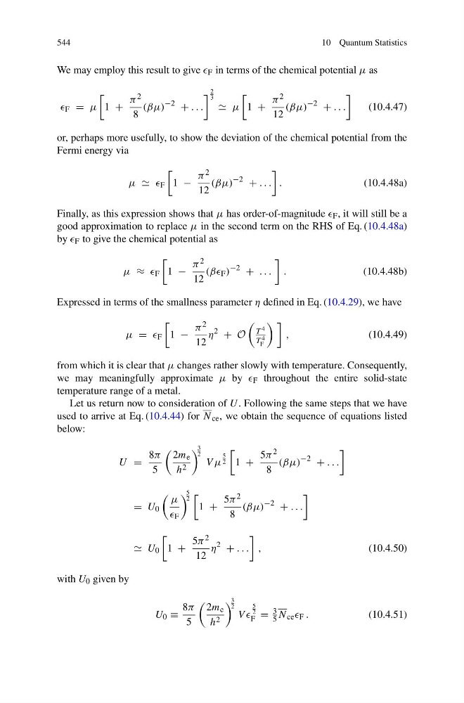
We may employ this result to give F in terms of the chemical potential μ as
F = μ
1 +
π 2
8
(βμ)
−2
+ . . .
2
3
μ
1 +
π 2
12
(βμ)
−2
+ . . .
(10.4.47)
or, perhaps more usefully, to show the deviation of the chemical potential from the
Fermi energy via
μ F
1 −
π 2
12
(βμ)
−2
+ . . .
.
(10.4.48a)
Finally, as this expression shows that μ has order-of-magnitude F , it will still be a
good approximation to replace μ in the second term on the RHS of Eq. (10.4.48a)
by F to give the chemical potential as
μ ≈ F
1 −
π 2
12
(ββ F )
−2
+ . . .
.
(10.4.48b)
Expressed in terms of the smallness parameter η defined in Eq. (10.4.29), we have
μ = F
1 −
π 2
12
η
2
+ O
T 4
T 4
F
,
(10.4.49)
from which it is clear that μ changes rather slowly with temperature. Consequently,
we may meaningfully approximate μ by F throughout the entire solid-state
temperature range of a metal.
Let us return now to consideration of U . Following the same steps that we have
used to arrive at Eq. (10.4.44) for N ce , we obtain the sequence of equations listed
below:
U =
8π
5
2m e
h 2
3
2
V μ
5
2
1 +
5π 2
8
(βμ)
−2
+ . . .
= U 0
μ
F
5
2
1 +
5π 2
8
(βμ)
−2
+ . . .
U 0
1 +
5π 2
12
η
2
+ . . .
,
(10.4.50)
with U 0 given by
U 0 ≡
8π
5
2m e
h 2
3
2
V V
5
2
F =
3
5 N ce F .
(10.4.51)
10 Quantum Statistics
We may employ this result to give F in terms of the chemical potential μ as
F = μ
1 +
π 2
8
(βμ)
−2
+ . . .
2
3
μ
1 +
π 2
12
(βμ)
−2
+ . . .
(10.4.47)
or, perhaps more usefully, to show the deviation of the chemical potential from the
Fermi energy via
μ F
1 −
π 2
12
(βμ)
−2
+ . . .
.
(10.4.48a)
Finally, as this expression shows that μ has order-of-magnitude F , it will still be a
good approximation to replace μ in the second term on the RHS of Eq. (10.4.48a)
by F to give the chemical potential as
μ ≈ F
1 −
π 2
12
(ββ F )
−2
+ . . .
.
(10.4.48b)
Expressed in terms of the smallness parameter η defined in Eq. (10.4.29), we have
μ = F
1 −
π 2
12
η
2
+ O
T 4
T 4
F
,
(10.4.49)
from which it is clear that μ changes rather slowly with temperature. Consequently,
we may meaningfully approximate μ by F throughout the entire solid-state
temperature range of a metal.
Let us return now to consideration of U . Following the same steps that we have
used to arrive at Eq. (10.4.44) for N ce , we obtain the sequence of equations listed
below:
U =
8π
5
2m e
h 2
3
2
V μ
5
2
1 +
5π 2
8
(βμ)
−2
+ . . .
= U 0
μ
F
5
2
1 +
5π 2
8
(βμ)
−2
+ . . .
U 0
1 +
5π 2
12
η
2
+ . . .
,
(10.4.50)
with U 0 given by
U 0 ≡
8π
5
2m e
h 2
3
2
V V
5
2
F =
3
5 N ce F .
(10.4.51)