

8.6 Magnetism, II. Ferromagnetism
469
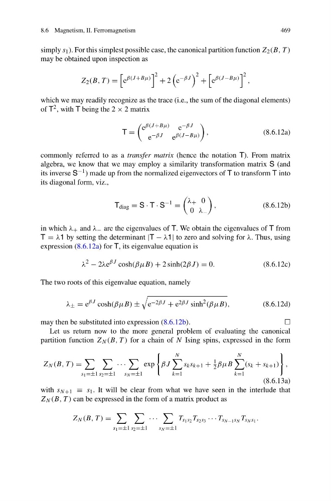
simply s 1 ). For this simplest possible case, the canonical partition function Z 2 (B, T )
may be obtained upon inspection as
Z 2 (B, T ) =
e
β(J +Bμ)
2 + 2
e
−βJ
2 +
e
β(J −Bμ)
2
,
which we may readily recognize as the trace (i.e., the sum of the diagonal elements)
of T 2 , with T being the 2 × 2 matrix
T =
e β(J +Bμ) e −βJ
e −βJ e β(J −Bμ)
,
(8.6.12a)
commonly referred to as a transfer matrix (hence the notation T). From matrix
algebra, we know that we may employ a similarity transformation matrix S (and
its inverse S −1 ) made up from the normalized eigenvectors of T to transform T into
its diagonal form, viz.,
T diag = S · T · S
−1
=
λ + 0
0 λ −
,
(8.6.12b)
in which λ + and λ − are the eigenvalues of T. We obtain the eigenvalues of T from
T = λ1 by setting the determinant |T − λ1| to zero and solving for λ. Thus, using
expression (8.6.12a) for T, its eigenvalue equation is
λ
2
− 2λe
βJ cosh(βμB) + 2 sinh(2βJ ) = 0.
(8.6.12c)
The two roots of this eigenvalue equation, namely
λ ± = e
βJ cosh(βμB) ±
e −2βJ + e 2βJ sinh
2 (βμB),
(8.6.12d)
may then be substituted into expression (8.6.12b).
Let us return now to the more general problem of evaluating the canonical
partition function Z N (B, T ) for a chain of N Ising spins, expressed in the form
Z N (B, T ) =
s 1 =±1
s 2 =±1
· · ·
s N =±1
exp
βJ
N
k=1
s k s k+1 +
1
2 βμB
N
k=1
(s k + s k+1 )
,
(8.6.13a)
with s N +1 ≡ s 1 . It will be clear from what we have seen in the interlude that
Z N (B, T ) can be expressed in the form of a matrix product as
Z N (B, T ) =
s 1 =±1
s 2 =±1
· · ·
s N =±1
T s 1 s 2 T s 2 s 3 · · · T s N−1 s N T s N s 1 .
469
simply s 1 ). For this simplest possible case, the canonical partition function Z 2 (B, T )
may be obtained upon inspection as
Z 2 (B, T ) =
e
β(J +Bμ)
2 + 2
e
−βJ
2 +
e
β(J −Bμ)
2
,
which we may readily recognize as the trace (i.e., the sum of the diagonal elements)
of T 2 , with T being the 2 × 2 matrix
T =
e β(J +Bμ) e −βJ
e −βJ e β(J −Bμ)
,
(8.6.12a)
commonly referred to as a transfer matrix (hence the notation T). From matrix
algebra, we know that we may employ a similarity transformation matrix S (and
its inverse S −1 ) made up from the normalized eigenvectors of T to transform T into
its diagonal form, viz.,
T diag = S · T · S
−1
=
λ + 0
0 λ −
,
(8.6.12b)
in which λ + and λ − are the eigenvalues of T. We obtain the eigenvalues of T from
T = λ1 by setting the determinant |T − λ1| to zero and solving for λ. Thus, using
expression (8.6.12a) for T, its eigenvalue equation is
λ
2
− 2λe
βJ cosh(βμB) + 2 sinh(2βJ ) = 0.
(8.6.12c)
The two roots of this eigenvalue equation, namely
λ ± = e
βJ cosh(βμB) ±
e −2βJ + e 2βJ sinh
2 (βμB),
(8.6.12d)
may then be substituted into expression (8.6.12b).
Let us return now to the more general problem of evaluating the canonical
partition function Z N (B, T ) for a chain of N Ising spins, expressed in the form
Z N (B, T ) =
s 1 =±1
s 2 =±1
· · ·
s N =±1
exp
βJ
N
k=1
s k s k+1 +
1
2 βμB
N
k=1
(s k + s k+1 )
,
(8.6.13a)
with s N +1 ≡ s 1 . It will be clear from what we have seen in the interlude that
Z N (B, T ) can be expressed in the form of a matrix product as
Z N (B, T ) =
s 1 =±1
s 2 =±1
· · ·
s N =±1
T s 1 s 2 T s 2 s 3 · · · T s N−1 s N T s N s 1 .