

452
8 Electric and Magnetic Phenomena
This is a fundamental relation for magnetic systems. Essentially the entire thermodynamics of magnetic systems can be derived from this rather important result,
taken together with Eq. (8.5.37) for the canonical partition function.
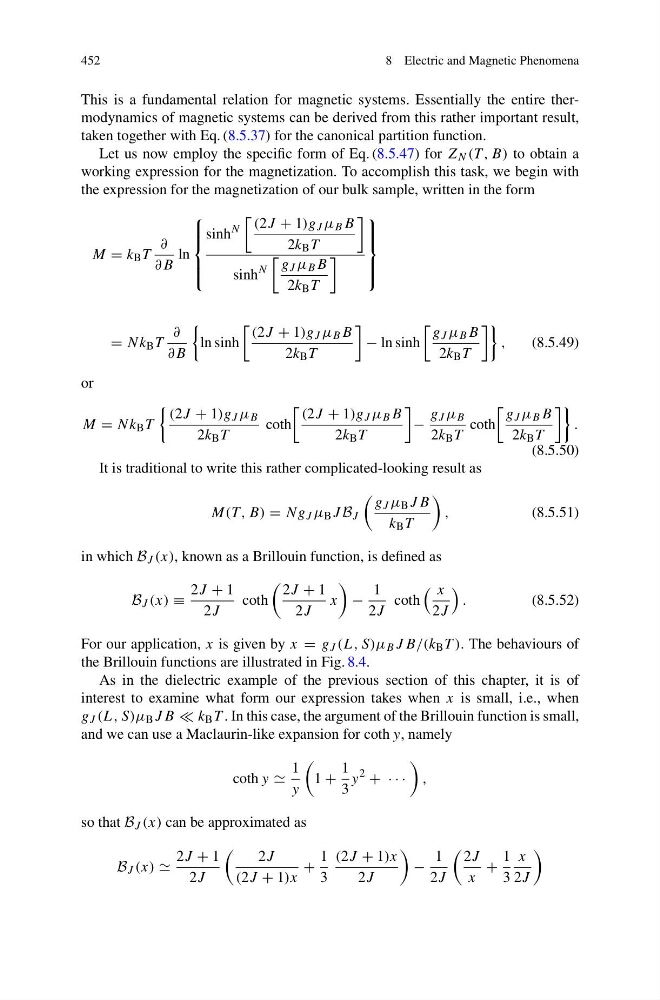
Let us now employ the specific form of Eq. (8.5.47) for Z N (T , B) to obtain a
working expression for the magnetization. To accomplish this task, we begin with
the expression for the magnetization of our bulk sample, written in the form
M = k B T
∂
∂B
ln
⎧
⎪ ⎪ ⎨
⎪ ⎪ ⎩
sinh
N
(2J + 1)g J μ B B
2k B T
sinh
N
g J μ B B
2k B T
⎫
⎪ ⎪ ⎬
⎪ ⎪ ⎭
= Nk B T
∂
∂B
ln sinh
(2J + 1)g J μ B B
2k B T
− ln sinh
g J μ B B
2k B T
,
(8.5.49)
or
M = Nk B T
(2J + 1)g J μ B
2k B T
coth
(2J + 1)g J μ B B
2k B T
−
g J μ B
2k B T
coth
g J μ B B
2k B T
.
(8.5.50)
It is traditional to write this rather complicated-looking result as
M(T , B) = Ng J μ B J B J
g J μ B J B
k B T
,
(8.5.51)
in which B J (x), known as a Brillouin function, is defined as
B J (x) ≡
2J + 1
2J
coth
2J + 1
2J
x
−
1
2J
coth
x
2J
.
(8.5.52)
For our application, x is given by x = g J (L, S)μ B J B/(k B T ). The behaviours of
the Brillouin functions are illustrated in Fig. 8.4.
As in the dielectric example of the previous section of this chapter, it is of
interest to examine what form our expression takes when x is small, i.e., when
g J (L, S)μ B J B k B T . In this case, the argument of the Brillouin function is small,
and we can use a Maclaurin-like expansion for coth y, namely
coth y
1
y
1 +
1
3
y
2
+ · · ·
,
so that B J (x) can be approximated as
B J (x)
2J + 1
2J
2J
(2J + 1)x
+
1
3
(2J + 1)x
2J
−
1
2J
2J
x
+
1
3
x
2J
8 Electric and Magnetic Phenomena
This is a fundamental relation for magnetic systems. Essentially the entire thermodynamics of magnetic systems can be derived from this rather important result,
taken together with Eq. (8.5.37) for the canonical partition function.
Let us now employ the specific form of Eq. (8.5.47) for Z N (T , B) to obtain a
working expression for the magnetization. To accomplish this task, we begin with
the expression for the magnetization of our bulk sample, written in the form
M = k B T
∂
∂B
ln
⎧
⎪ ⎪ ⎨
⎪ ⎪ ⎩
sinh
N
(2J + 1)g J μ B B
2k B T
sinh
N
g J μ B B
2k B T
⎫
⎪ ⎪ ⎬
⎪ ⎪ ⎭
= Nk B T
∂
∂B
ln sinh
(2J + 1)g J μ B B
2k B T
− ln sinh
g J μ B B
2k B T
,
(8.5.49)
or
M = Nk B T
(2J + 1)g J μ B
2k B T
coth
(2J + 1)g J μ B B
2k B T
−
g J μ B
2k B T
coth
g J μ B B
2k B T
.
(8.5.50)
It is traditional to write this rather complicated-looking result as
M(T , B) = Ng J μ B J B J
g J μ B J B
k B T
,
(8.5.51)
in which B J (x), known as a Brillouin function, is defined as
B J (x) ≡
2J + 1
2J
coth
2J + 1
2J
x
−
1
2J
coth
x
2J
.
(8.5.52)
For our application, x is given by x = g J (L, S)μ B J B/(k B T ). The behaviours of
the Brillouin functions are illustrated in Fig. 8.4.
As in the dielectric example of the previous section of this chapter, it is of
interest to examine what form our expression takes when x is small, i.e., when
g J (L, S)μ B J B k B T . In this case, the argument of the Brillouin function is small,
and we can use a Maclaurin-like expansion for coth y, namely
coth y
1
y
1 +
1
3
y
2
+ · · ·
,
so that B J (x) can be approximated as
B J (x)
2J + 1
2J
2J
(2J + 1)x
+
1
3
(2J + 1)x
2J
−
1
2J
2J
x
+
1
3
x
2J