

382
7 Classical Statistical Mechanics
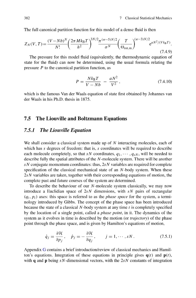
The full canonical partition function for this model of a dense fluid is then
Z N (V , T ) =
(V −Nb) N
N!
2πMk B T
h 2
3N/2 π (w−5)N/2
σ N
T
rot,m
(w−3)N/2
e
aN 2 /(V k B T ) .
(7.4.9)
The pressure for this model fluid (equivalently, the thermodynamic equation of
state for the fluid) can now be determined, using the usual formula relating the
pressure P to the canonical partition function, as
P =
Nk B T
V − Nb
−
aN 2
V 2 ,
(7.4.10)
which is the famous Van der Waals equation of state first obtained by Johannes van
der Waals in his Ph.D. thesis in 1875.
7.5 The Liouville and Boltzmann Equations
7.5.1 The Liouville Equation
We shall consider a classical system made up of N interacting molecules, each of
which has s degrees of freedom: that is, s coordinates will be required to describe
each molecule completely, so that sN coordinates, q 1 , · · · , q sN , will be needed to
describe fully the spatial attributes of the N-molecule system. There will be another
sN conjugate momentum coordinates: thus, 2sN variables are required for complete
specification of the classical mechanical state of an N-body system. When these
2sN variables are taken, together with their corresponding equations of motion, the
complete past and future courses of the system are determined.
To describe the behaviour of our N-molecule system classically, we may now
introduce a Euclidian space of 2sN dimensions, with sN pairs of rectangular
(q i , p i ) axes: this space is referred to as the phase space for the system, a terminology introduced by Gibbs. The concept of the phase space has been introduced
because the state of a classical N-body system at any time t is completely specified
by the location of a single point, called a phase point, in it. The dynamics of the
system as it evolves in time is described by the motion (or trajectory) of the phase
point through the phase space, and is given by Hamilton’s equations of motion,
˙
q j =
∂H
∂p j
, ˙
p j = −
∂H
∂q j
,
j = 1, · · · , sN .
(7.5.1)
Appendix G contains a brief introduction/review of classical mechanics and Hamilton’s equations. Integration of these equations in principle gives q(t) and p(t),
with q and p being sN-dimensional vectors, with the 2sN constants of integration
7 Classical Statistical Mechanics
The full canonical partition function for this model of a dense fluid is then
Z N (V , T ) =
(V −Nb) N
N!
2πMk B T
h 2
3N/2 π (w−5)N/2
σ N
T
rot,m
(w−3)N/2
e
aN 2 /(V k B T ) .
(7.4.9)
The pressure for this model fluid (equivalently, the thermodynamic equation of
state for the fluid) can now be determined, using the usual formula relating the
pressure P to the canonical partition function, as
P =
Nk B T
V − Nb
−
aN 2
V 2 ,
(7.4.10)
which is the famous Van der Waals equation of state first obtained by Johannes van
der Waals in his Ph.D. thesis in 1875.
7.5 The Liouville and Boltzmann Equations
7.5.1 The Liouville Equation
We shall consider a classical system made up of N interacting molecules, each of
which has s degrees of freedom: that is, s coordinates will be required to describe
each molecule completely, so that sN coordinates, q 1 , · · · , q sN , will be needed to
describe fully the spatial attributes of the N-molecule system. There will be another
sN conjugate momentum coordinates: thus, 2sN variables are required for complete
specification of the classical mechanical state of an N-body system. When these
2sN variables are taken, together with their corresponding equations of motion, the
complete past and future courses of the system are determined.
To describe the behaviour of our N-molecule system classically, we may now
introduce a Euclidian space of 2sN dimensions, with sN pairs of rectangular
(q i , p i ) axes: this space is referred to as the phase space for the system, a terminology introduced by Gibbs. The concept of the phase space has been introduced
because the state of a classical N-body system at any time t is completely specified
by the location of a single point, called a phase point, in it. The dynamics of the
system as it evolves in time is described by the motion (or trajectory) of the phase
point through the phase space, and is given by Hamilton’s equations of motion,
˙
q j =
∂H
∂p j
, ˙
p j = −
∂H
∂q j
,
j = 1, · · · , sN .
(7.5.1)
Appendix G contains a brief introduction/review of classical mechanics and Hamilton’s equations. Integration of these equations in principle gives q(t) and p(t),
with q and p being sN-dimensional vectors, with the 2sN constants of integration