

120
2 Macroscopic Thermodynamics
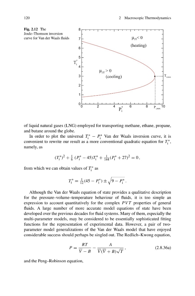
Fig. 2.12 The
Joule–Thomson inversion
curve for Van der Waals fluids
0
2
4
6
8
10
0
1
2
3
4
5
6
7
8
P i
*
T i
*
μ JT > 0
μ JT < 0
(cooling)
(heating)
T i,max
P i,max
of liquid natural gases (LNG) employed for transporting methane, ethane, propane,
and butane around the globe.
In order to plot the universal T ∗
i − P ∗
i Van der Waals inversion curve, it is
convenient to rewrite our result as a more conventional quadratic equation for T ∗
i ,
namely, as
(T
∗
i )
2
+
1
6 (P
∗
i − 45)T
∗
i +
1
144 (P
∗
i + 27)
2
= 0 ,
from which we can obtain values of T ∗
i as
T
∗
i =
1
12 (45 − P
∗
i ) ±
9 − P ∗
i .
Although the Van der Waals equation of state provides a qualitative description
for the pressure–volume–temperature behaviour of fluids, it is too simple an
expression to account quantitatively for the complex P V T properties of general
fluids. A large number of more accurate model equations of state have been
developed over the previous decades for fluid systems. Many of them, especially the
multi-parameter models, may be considered to be essentially sophisticated fitting
functions for the representation of experimental data. However, a pair of twoparameter model generalizations of the Van der Waals model that have enjoyed
considerable success should perhaps be singled out. The Redlich–Kwong equation,
P =
RT
V − B
−
A
V (V + B)
√
T
,
(2.8.36a)
and the Peng–Robinson equation,
2 Macroscopic Thermodynamics
Fig. 2.12 The
Joule–Thomson inversion
curve for Van der Waals fluids
0
2
4
6
8
10
0
1
2
3
4
5
6
7
8
P i
*
T i
*
μ JT > 0
μ JT < 0
(cooling)
(heating)
T i,max
P i,max
of liquid natural gases (LNG) employed for transporting methane, ethane, propane,
and butane around the globe.
In order to plot the universal T ∗
i − P ∗
i Van der Waals inversion curve, it is
convenient to rewrite our result as a more conventional quadratic equation for T ∗
i ,
namely, as
(T
∗
i )
2
+
1
6 (P
∗
i − 45)T
∗
i +
1
144 (P
∗
i + 27)
2
= 0 ,
from which we can obtain values of T ∗
i as
T
∗
i =
1
12 (45 − P
∗
i ) ±
9 − P ∗
i .
Although the Van der Waals equation of state provides a qualitative description
for the pressure–volume–temperature behaviour of fluids, it is too simple an
expression to account quantitatively for the complex P V T properties of general
fluids. A large number of more accurate model equations of state have been
developed over the previous decades for fluid systems. Many of them, especially the
multi-parameter models, may be considered to be essentially sophisticated fitting
functions for the representation of experimental data. However, a pair of twoparameter model generalizations of the Van der Waals model that have enjoyed
considerable success should perhaps be singled out. The Redlich–Kwong equation,
P =
RT
V − B
−
A
V (V + B)
√
T
,
(2.8.36a)
and the Peng–Robinson equation,