

1.6 Dynamics of Magnetic Moments: Landau-Lifshitz-Gilbert Equation
13
L =
m
γ ,
(1.19)
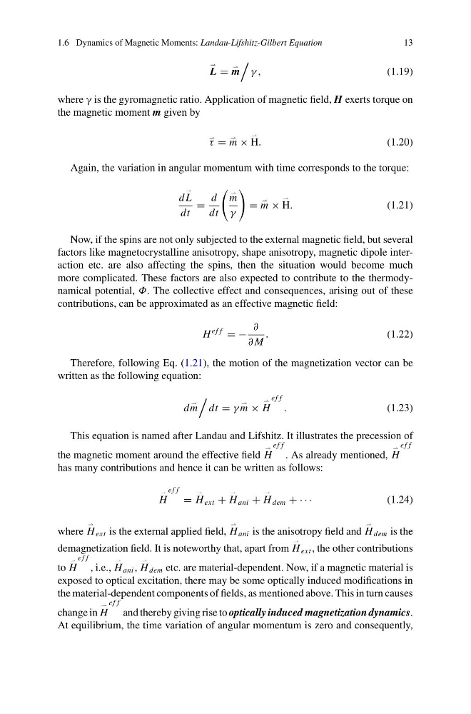
where γ is the gyromagnetic ratio. Application of magnetic field, H exerts torque on
the magnetic moment m given by
τ =
m ×
H.
(1.20)
Again, the variation in angular momentum with time corresponds to the torque:
d
L
dt
=
d
dt
m
γ
=
m ×
H.
(1.21)
Now, if the spins are not only subjected to the external magnetic field, but several
factors like magnetocrystalline anisotropy, shape anisotropy, magnetic dipole interaction etc. are also affecting the spins, then the situation would become much
more complicated. These factors are also expected to contribute to the thermodynamical potential, Φ. The collective effect and consequences, arising out of these
contributions, can be approximated as an effective magnetic field:
H
e f f
= −
∂
∂ M
.
(1.22)
Therefore, following Eq. (1.21), the motion of the magnetization vector can be
written as the following equation:
d
m
dt = γ
m ×
H
e f f
.
(1.23)
This equation is named after Landau and Lifshitz. It illustrates the precession of
the magnetic moment around the effective field
H
e f f
. As already mentioned,
H
e f f
has many contributions and hence it can be written as follows:
H
e f f
=
H ext +
H ani +
H dem + · · ·
(1.24)
where
H ext is the external applied field,
H ani is the anisotropy field and
H dem is the
demagnetization field. It is noteworthy that, apart from
H ext , the other contributions
to
H
e f f
, i.e.,
H ani ,
H dem etc. are material-dependent. Now, if a magnetic material is
exposed to optical excitation, there may be some optically induced modifications in
the material-dependent components of fields, as mentioned above. This in turn causes
change in
H
e f f
and thereby giving rise to optically induced magnetization dynamics.
At equilibrium, the time variation of angular momentum is zero and consequently,
13
L =
m
γ ,
(1.19)
where γ is the gyromagnetic ratio. Application of magnetic field, H exerts torque on
the magnetic moment m given by
τ =
m ×
H.
(1.20)
Again, the variation in angular momentum with time corresponds to the torque:
d
L
dt
=
d
dt
m
γ
=
m ×
H.
(1.21)
Now, if the spins are not only subjected to the external magnetic field, but several
factors like magnetocrystalline anisotropy, shape anisotropy, magnetic dipole interaction etc. are also affecting the spins, then the situation would become much
more complicated. These factors are also expected to contribute to the thermodynamical potential, Φ. The collective effect and consequences, arising out of these
contributions, can be approximated as an effective magnetic field:
H
e f f
= −
∂
∂ M
.
(1.22)
Therefore, following Eq. (1.21), the motion of the magnetization vector can be
written as the following equation:
d
m
dt = γ
m ×
H
e f f
.
(1.23)
This equation is named after Landau and Lifshitz. It illustrates the precession of
the magnetic moment around the effective field
H
e f f
. As already mentioned,
H
e f f
has many contributions and hence it can be written as follows:
H
e f f
=
H ext +
H ani +
H dem + · · ·
(1.24)
where
H ext is the external applied field,
H ani is the anisotropy field and
H dem is the
demagnetization field. It is noteworthy that, apart from
H ext , the other contributions
to
H
e f f
, i.e.,
H ani ,
H dem etc. are material-dependent. Now, if a magnetic material is
exposed to optical excitation, there may be some optically induced modifications in
the material-dependent components of fields, as mentioned above. This in turn causes
change in
H
e f f
and thereby giving rise to optically induced magnetization dynamics.
At equilibrium, the time variation of angular momentum is zero and consequently,