

12
1 An Overview of Spintronics
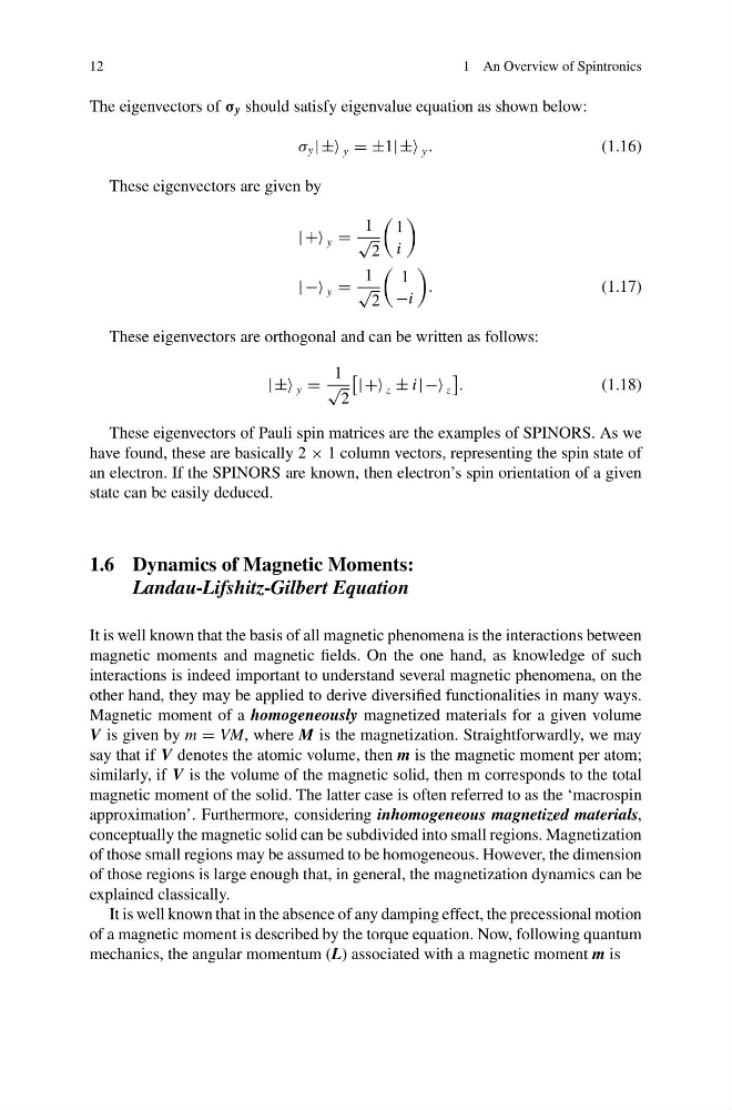
The eigenvectors of σ y should satisfy eigenvalue equation as shown below:
σ y | ± y = ±1| ± y .
(1.16)
These eigenvectors are given by
| + y =
1
√
2
1
i
| − y =
1
√
2
1
−i
.
(1.17)
These eigenvectors are orthogonal and can be written as follows:
| ± y =
1
√
2
| + z ± i| − z
.
(1.18)
These eigenvectors of Pauli spin matrices are the examples of SPINORS. As we
have found, these are basically 2 × 1 column vectors, representing the spin state of
an electron. If the SPINORS are known, then electron’s spin orientation of a given
state can be easily deduced.
1.6 Dynamics of Magnetic Moments:
Landau-Lifshitz-Gilbert Equation
It is well known that the basis of all magnetic phenomena is the interactions between
magnetic moments and magnetic fields. On the one hand, as knowledge of such
interactions is indeed important to understand several magnetic phenomena, on the
other hand, they may be applied to derive diversified functionalities in many ways.
Magnetic moment of a homogeneously magnetized materials for a given volume
V is given by m = VM, where M is the magnetization. Straightforwardly, we may
say that if V denotes the atomic volume, then m is the magnetic moment per atom;
similarly, if V is the volume of the magnetic solid, then m corresponds to the total
magnetic moment of the solid. The latter case is often referred to as the ‘macrospin
approximation’. Furthermore, considering inhomogeneous magnetized materials,
conceptually the magnetic solid can be subdivided into small regions. Magnetization
of those small regions may be assumed to be homogeneous. However, the dimension
of those regions is large enough that, in general, the magnetization dynamics can be
explained classically.
It is well known that in the absence of any damping effect, the precessional motion
of a magnetic moment is described by the torque equation. Now, following quantum
mechanics, the angular momentum (L) associated with a magnetic moment m is
1 An Overview of Spintronics
The eigenvectors of σ y should satisfy eigenvalue equation as shown below:
σ y | ± y = ±1| ± y .
(1.16)
These eigenvectors are given by
| + y =
1
√
2
1
i
| − y =
1
√
2
1
−i
.
(1.17)
These eigenvectors are orthogonal and can be written as follows:
| ± y =
1
√
2
| + z ± i| − z
.
(1.18)
These eigenvectors of Pauli spin matrices are the examples of SPINORS. As we
have found, these are basically 2 × 1 column vectors, representing the spin state of
an electron. If the SPINORS are known, then electron’s spin orientation of a given
state can be easily deduced.
1.6 Dynamics of Magnetic Moments:
Landau-Lifshitz-Gilbert Equation
It is well known that the basis of all magnetic phenomena is the interactions between
magnetic moments and magnetic fields. On the one hand, as knowledge of such
interactions is indeed important to understand several magnetic phenomena, on the
other hand, they may be applied to derive diversified functionalities in many ways.
Magnetic moment of a homogeneously magnetized materials for a given volume
V is given by m = VM, where M is the magnetization. Straightforwardly, we may
say that if V denotes the atomic volume, then m is the magnetic moment per atom;
similarly, if V is the volume of the magnetic solid, then m corresponds to the total
magnetic moment of the solid. The latter case is often referred to as the ‘macrospin
approximation’. Furthermore, considering inhomogeneous magnetized materials,
conceptually the magnetic solid can be subdivided into small regions. Magnetization
of those small regions may be assumed to be homogeneous. However, the dimension
of those regions is large enough that, in general, the magnetization dynamics can be
explained classically.
It is well known that in the absence of any damping effect, the precessional motion
of a magnetic moment is described by the torque equation. Now, following quantum
mechanics, the angular momentum (L) associated with a magnetic moment m is