

2.5 Normalization
65
A proper account requires to gauge fix this symmetry: the simplest possibility is to
insert three or more vertex operators—this topic is discussed in Sect. 3.1.
Finally, note that the same question arises for the b-ghost since one has the
symmetry
b −→ b + b 0 ,
P
†
1 b 0 = 0.
(2.165)
That there is no problem in this case is related to the presence of the moduli.
2.5
Normalization
In the previous sections, the closed string coupling constant g s did not appear in
the expressions. Loops in vacuum amplitudes are generated by splitting of closed
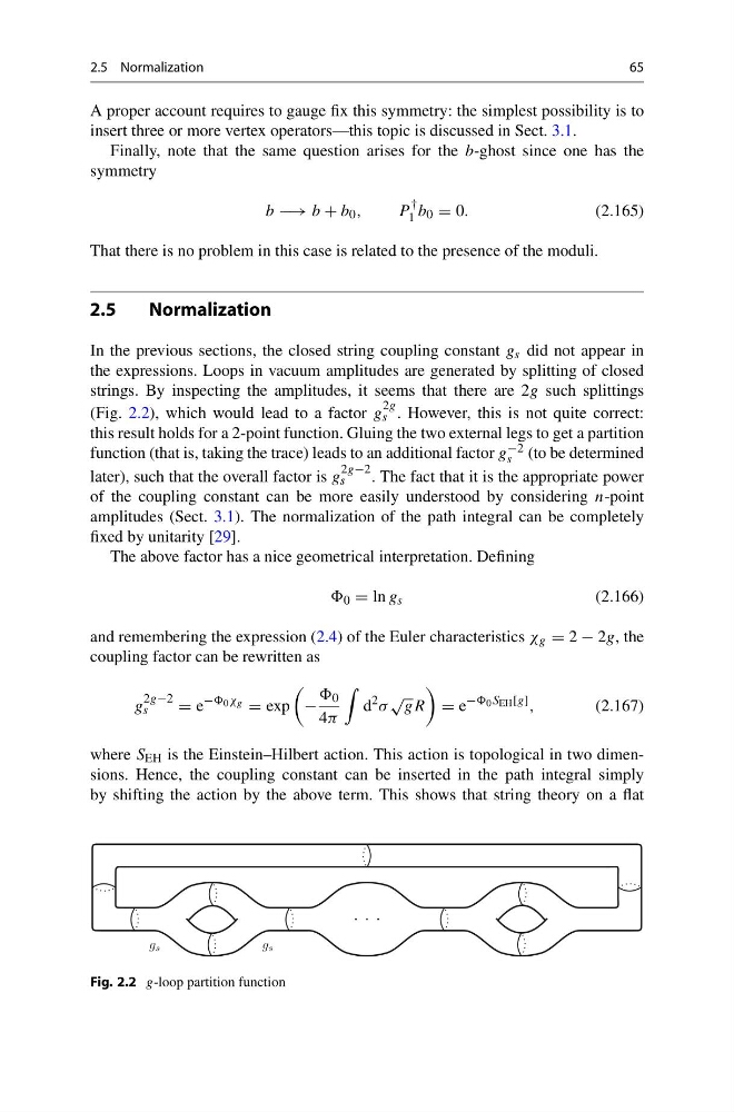
strings. By inspecting the amplitudes, it seems that there are 2g such splittings
(Fig. 2.2), which would lead to a factor g
2g
s . However, this is not quite correct:
this result holds for a 2-point function. Gluing the two external legs to get a partition
function (that is, taking the trace) leads to an additional factor g −2
s (to be determined
later), such that the overall factor is g
2g−2
s
. The fact that it is the appropriate power
of the coupling constant can be more easily understood by considering n-point
amplitudes (Sect. 3.1). The normalization of the path integral can be completely
fixed by unitarity [29].
The above factor has a nice geometrical interpretation. Defining
0 = ln g s
(2.166)
and remembering the expression (2.4) of the Euler characteristics χ g = 2 − 2g, the
coupling factor can be rewritten as
g
2g−2
s
= e
− 0 χ g = exp
−
0
4π
d
2 σ
√
gR
= e
− 0 S EH [g] ,
(2.167)
where S EH is the Einstein–Hilbert action. This action is topological in two dimensions. Hence, the coupling constant can be inserted in the path integral simply
by shifting the action by the above term. This shows that string theory on a flat
Fig. 2.2 g-loop partition function
65
A proper account requires to gauge fix this symmetry: the simplest possibility is to
insert three or more vertex operators—this topic is discussed in Sect. 3.1.
Finally, note that the same question arises for the b-ghost since one has the
symmetry
b −→ b + b 0 ,
P
†
1 b 0 = 0.
(2.165)
That there is no problem in this case is related to the presence of the moduli.
2.5
Normalization
In the previous sections, the closed string coupling constant g s did not appear in
the expressions. Loops in vacuum amplitudes are generated by splitting of closed
strings. By inspecting the amplitudes, it seems that there are 2g such splittings
(Fig. 2.2), which would lead to a factor g
2g
s . However, this is not quite correct:
this result holds for a 2-point function. Gluing the two external legs to get a partition
function (that is, taking the trace) leads to an additional factor g −2
s (to be determined
later), such that the overall factor is g
2g−2
s
. The fact that it is the appropriate power
of the coupling constant can be more easily understood by considering n-point
amplitudes (Sect. 3.1). The normalization of the path integral can be completely
fixed by unitarity [29].
The above factor has a nice geometrical interpretation. Defining
0 = ln g s
(2.166)
and remembering the expression (2.4) of the Euler characteristics χ g = 2 − 2g, the
coupling factor can be rewritten as
g
2g−2
s
= e
− 0 χ g = exp
−
0
4π
d
2 σ
√
gR
= e
− 0 S EH [g] ,
(2.167)
where S EH is the Einstein–Hilbert action. This action is topological in two dimensions. Hence, the coupling constant can be inserted in the path integral simply
by shifting the action by the above term. This shows that string theory on a flat
Fig. 2.2 g-loop partition function