

2.3 Faddeev–Popov Gauge Fixing
47
(these should not be confused with the Liouville field). The dimension of ker P
†
1 is
in fact equal to the dimension of the moduli space (2.51):
dim R ker P
†
1 = M g =
⎧
⎪ ⎪ ⎨
⎪ ⎪ ⎩
0
g = 0,
2
g = 1,
6g − 6 g > 1.
(2.77)
The last two terms in the variation (2.64) of δg ab are not orthogonal. Let us
introduce the projector on the complement space of ker P
†
1
:= P 1
1
P
†
1 P 1
P
†
1 .
(2.78)
The moduli variations can then be rewritten as
δt i μ i = δt i (1 − )μ i + δt i μ i = δt i (1 − )μ i + δt i P 1 ζ i .
(2.79)
The ζ i exist because μ i ∈ Im P 1 , and they read
ζ i :=
1
P
†
1 P 1
P
†
1 μ i .
(2.80)
The first term can be decomposed on the quadratic differential basis (2.76)
(1 − )μ i = φ j (M
−1 ) jk (φ k , μ i ) g ,
(2.81)
where
M ij := (φ i , φ j ) g .
(2.82)
Ultimately, the variation (2.64) becomes
δg ab = (P 1 ˜
ξ) ab + 2 ˜
g ab + Q iab δt i .
(2.83)
where
˜
ξ = ξ + ζ i δt i ,
Q iab = φ jab (M
−1 ) jk (φ k , μ i ) g .
(2.84)
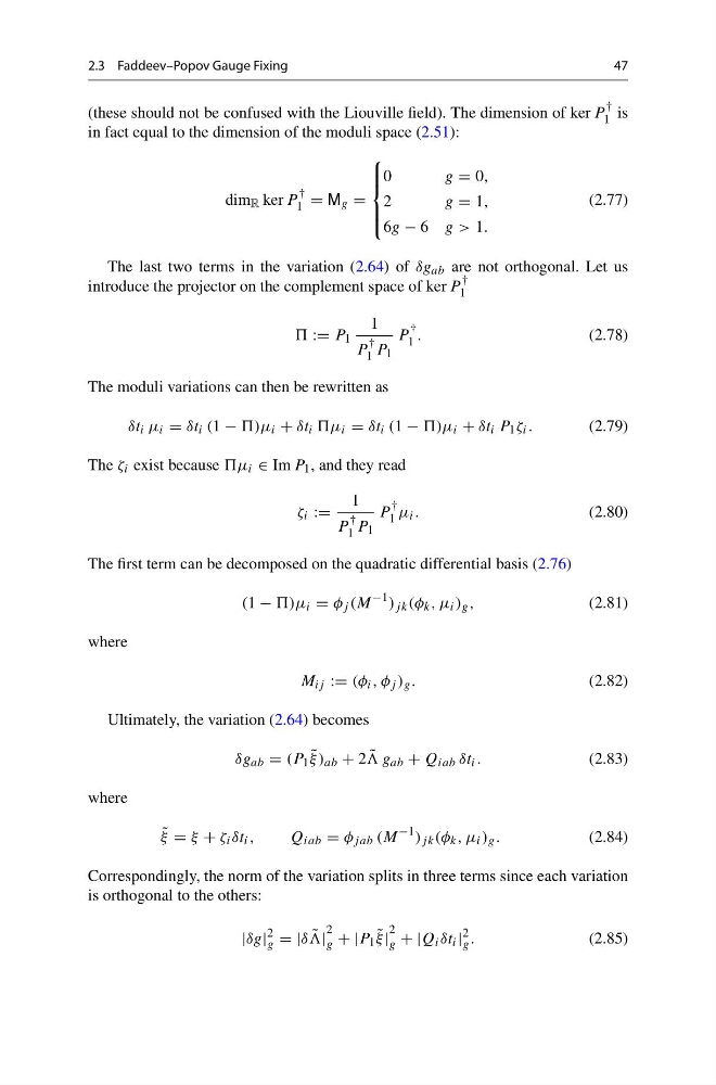
Correspondingly, the norm of the variation splits in three terms since each variation
is orthogonal to the others:
|δg|
2
g = |δ ˜
|
2
g + |P 1 ˜
ξ |
2
g + |Q i δt i |
2
g .
(2.85)
47
(these should not be confused with the Liouville field). The dimension of ker P
†
1 is
in fact equal to the dimension of the moduli space (2.51):
dim R ker P
†
1 = M g =
⎧
⎪ ⎪ ⎨
⎪ ⎪ ⎩
0
g = 0,
2
g = 1,
6g − 6 g > 1.
(2.77)
The last two terms in the variation (2.64) of δg ab are not orthogonal. Let us
introduce the projector on the complement space of ker P
†
1
:= P 1
1
P
†
1 P 1
P
†
1 .
(2.78)
The moduli variations can then be rewritten as
δt i μ i = δt i (1 − )μ i + δt i μ i = δt i (1 − )μ i + δt i P 1 ζ i .
(2.79)
The ζ i exist because μ i ∈ Im P 1 , and they read
ζ i :=
1
P
†
1 P 1
P
†
1 μ i .
(2.80)
The first term can be decomposed on the quadratic differential basis (2.76)
(1 − )μ i = φ j (M
−1 ) jk (φ k , μ i ) g ,
(2.81)
where
M ij := (φ i , φ j ) g .
(2.82)
Ultimately, the variation (2.64) becomes
δg ab = (P 1 ˜
ξ) ab + 2 ˜
g ab + Q iab δt i .
(2.83)
where
˜
ξ = ξ + ζ i δt i ,
Q iab = φ jab (M
−1 ) jk (φ k , μ i ) g .
(2.84)
Correspondingly, the norm of the variation splits in three terms since each variation
is orthogonal to the others:
|δg|
2
g = |δ ˜
|
2
g + |P 1 ˜
ξ |
2
g + |Q i δt i |
2
g .
(2.85)