

2.1 Worldsheet Action and Symmetries
33
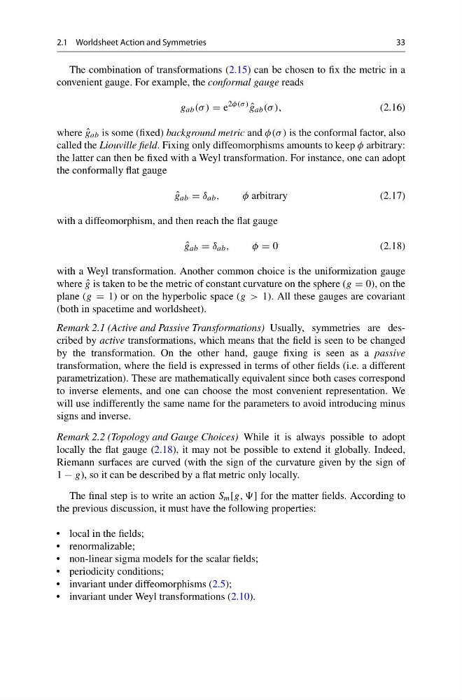
The combination of transformations (2.15) can be chosen to fix the metric in a
convenient gauge. For example, the conformal gauge reads
g ab (σ ) = e
2φ(σ )
ˆ
g ab (σ ),
(2.16)
where ˆ
g ab is some (fixed) background metric and φ(σ ) is the conformal factor, also
called the Liouville field. Fixing only diffeomorphisms amounts to keep φ arbitrary:
the latter can then be fixed with a Weyl transformation. For instance, one can adopt
the conformally flat gauge
ˆ
g ab = δ ab ,
φarbitrary
(2.17)
with a diffeomorphism, and then reach the flat gauge
ˆ
g ab = δ ab ,
φ = 0
(2.18)
with a Weyl transformation. Another common choice is the uniformization gauge
where ˆ
g is taken to be the metric of constant curvature on the sphere (g = 0), on the
plane (g = 1) or on the hyperbolic space (g > 1). All these gauges are covariant
(both in spacetime and worldsheet).
Remark 2.1 (Active and Passive Transformations) Usually, symmetries are described by active transformations, which means that the field is seen to be changed
by the transformation. On the other hand, gauge fixing is seen as a passive
transformation, where the field is expressed in terms of other fields (i.e. a different
parametrization). These are mathematically equivalent since both cases correspond
to inverse elements, and one can choose the most convenient representation. We
will use indifferently the same name for the parameters to avoid introducing minus
signs and inverse.
Remark 2.2 (Topology and Gauge Choices) While it is always possible to adopt
locally the flat gauge (2.18), it may not be possible to extend it globally. Indeed,
Riemann surfaces are curved (with the sign of the curvature given by the sign of
1 − g), so it can be described by a flat metric only locally.
The final step is to write an action S m [g, ,] for the matter fields. According to
the previous discussion, it must have the following properties:
• local in the fields;
• renormalizable;
• non-linear sigma models for the scalar fields;
• periodicity conditions;
• invariant under diffeomorphisms (2.5);
• invariant under Weyl transformations (2.10).
33
The combination of transformations (2.15) can be chosen to fix the metric in a
convenient gauge. For example, the conformal gauge reads
g ab (σ ) = e
2φ(σ )
ˆ
g ab (σ ),
(2.16)
where ˆ
g ab is some (fixed) background metric and φ(σ ) is the conformal factor, also
called the Liouville field. Fixing only diffeomorphisms amounts to keep φ arbitrary:
the latter can then be fixed with a Weyl transformation. For instance, one can adopt
the conformally flat gauge
ˆ
g ab = δ ab ,
φarbitrary
(2.17)
with a diffeomorphism, and then reach the flat gauge
ˆ
g ab = δ ab ,
φ = 0
(2.18)
with a Weyl transformation. Another common choice is the uniformization gauge
where ˆ
g is taken to be the metric of constant curvature on the sphere (g = 0), on the
plane (g = 1) or on the hyperbolic space (g > 1). All these gauges are covariant
(both in spacetime and worldsheet).
Remark 2.1 (Active and Passive Transformations) Usually, symmetries are described by active transformations, which means that the field is seen to be changed
by the transformation. On the other hand, gauge fixing is seen as a passive
transformation, where the field is expressed in terms of other fields (i.e. a different
parametrization). These are mathematically equivalent since both cases correspond
to inverse elements, and one can choose the most convenient representation. We
will use indifferently the same name for the parameters to avoid introducing minus
signs and inverse.
Remark 2.2 (Topology and Gauge Choices) While it is always possible to adopt
locally the flat gauge (2.18), it may not be possible to extend it globally. Indeed,
Riemann surfaces are curved (with the sign of the curvature given by the sign of
1 − g), so it can be described by a flat metric only locally.
The final step is to write an action S m [g, ,] for the matter fields. According to
the previous discussion, it must have the following properties:
• local in the fields;
• renormalizable;
• non-linear sigma models for the scalar fields;
• periodicity conditions;
• invariant under diffeomorphisms (2.5);
• invariant under Weyl transformations (2.10).