

408
C Quantum Field Theory
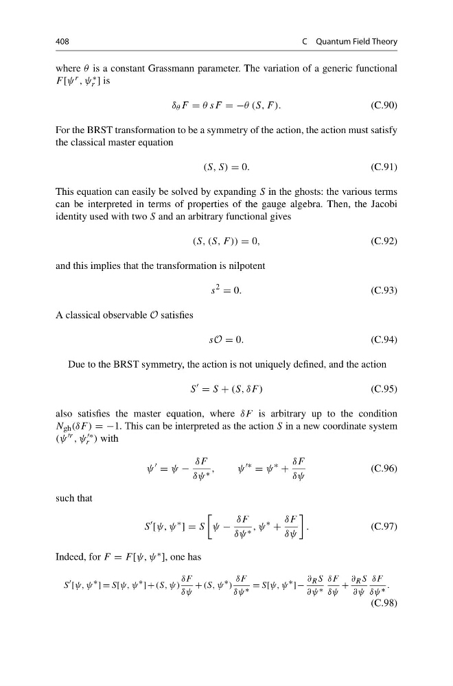
where θ is a constant Grassmann parameter. The variation of a generic functional
F [ψ r , ψ ∗
r ] is
δ θ F = θ sF = −θ (S, F ).
(C.90)
For the BRST transformation to be a symmetry of the action, the action must satisfy
the classical master equation
(S, S) = 0.
(C.91)
This equation can easily be solved by expanding S in the ghosts: the various terms
can be interpreted in terms of properties of the gauge algebra. Then, the Jacobi
identity used with two S and an arbitrary functional gives
(S, (S, F )) = 0,
(C.92)
and this implies that the transformation is nilpotent
s
2
= 0.
(C.93)
A classical observable O satisfies
sO = 0.
(C.94)
Due to the BRST symmetry, the action is not uniquely defined, and the action
S
= S + (S, δF )
(C.95)
also satisfies the master equation, where δF is arbitrary up to the condition
N gh (δF ) = −1. This can be interpreted as the action S in a new coordinate system
(ψ r , ψ ∗
r ) with
ψ
= ψ −
δF
δψ ∗ ,
ψ
∗
= ψ
∗
+
δF
δψ
(C.96)
such that
S
[ψ, ψ
∗
] = S
ψ −
δF
δψ ∗ , ψ
∗
+
δF
δψ
.
(C.97)
Indeed, for F = F [ψ, ψ ∗ ], one has
S [ψ, ψ ∗ ] = S[ψ, ψ ∗ ]+(S, ψ)
δF
δψ
+ (S, ψ ∗ )
δF
δψ ∗ = S[ψ, ψ ∗ ]−
∂ R S
∂ψ ∗
δF
δψ
+
∂ R S
∂ψ
δF
δψ ∗ .
(C.98)
C Quantum Field Theory
where θ is a constant Grassmann parameter. The variation of a generic functional
F [ψ r , ψ ∗
r ] is
δ θ F = θ sF = −θ (S, F ).
(C.90)
For the BRST transformation to be a symmetry of the action, the action must satisfy
the classical master equation
(S, S) = 0.
(C.91)
This equation can easily be solved by expanding S in the ghosts: the various terms
can be interpreted in terms of properties of the gauge algebra. Then, the Jacobi
identity used with two S and an arbitrary functional gives
(S, (S, F )) = 0,
(C.92)
and this implies that the transformation is nilpotent
s
2
= 0.
(C.93)
A classical observable O satisfies
sO = 0.
(C.94)
Due to the BRST symmetry, the action is not uniquely defined, and the action
S
= S + (S, δF )
(C.95)
also satisfies the master equation, where δF is arbitrary up to the condition
N gh (δF ) = −1. This can be interpreted as the action S in a new coordinate system
(ψ r , ψ ∗
r ) with
ψ
= ψ −
δF
δψ ∗ ,
ψ
∗
= ψ
∗
+
δF
δψ
(C.96)
such that
S
[ψ, ψ
∗
] = S
ψ −
δF
δψ ∗ , ψ
∗
+
δF
δψ
.
(C.97)
Indeed, for F = F [ψ, ψ ∗ ], one has
S [ψ, ψ ∗ ] = S[ψ, ψ ∗ ]+(S, ψ)
δF
δψ
+ (S, ψ ∗ )
δF
δψ ∗ = S[ψ, ψ ∗ ]−
∂ R S
∂ψ ∗
δF
δψ
+
∂ R S
∂ψ
δF
δψ ∗ .
(C.98)