

17.2 Off-Shell Superstring Amplitudes
351
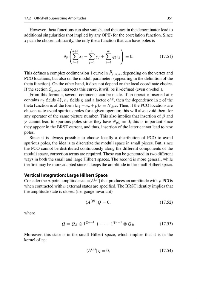
However, theta functions can also vanish, and the ones in the denominator lead to
additional singularities (not implied by any OPE) for the correlation function. Since
x 1 can be chosen arbitrarily, the only theta function that can have poles is
ϑ δ
⎛
⎝
n+1
i=2
x i −
n
j =1
y j +
m
k=1
q k z k
⎞
⎠ = 0.
(17.51)
This defines a complex codimension 1 curve in
P g,m,n , depending on the vertex and
PCO locations, but also on the moduli parameters (appearing in the definition of the
theta function). On the other hand, it does not depend on the local coordinate choice.
If the section S g,m,n intersects this curve, it will be ill-defined (even on-shell).
From this formula, several comments can be made. If an operator inserted at z
contains n ξ fields ∂ξ , n η fields η and a factor e pφ , then the dependence in z of the
theta function is of the form (n ξ − n η + p)z = N pic z. Then, if the PCO locations are
chosen as to avoid spurious poles for a given operator, this will also avoid them for
any operator of the same picture number. This also implies that insertion of β and
γ cannot lead to spurious poles since they have N pic = 0; this is important since
they appear in the BRST current, and thus, insertion of the latter cannot lead to new
poles.
Since it is always possible to choose locally a distribution of PCO to avoid
spurious poles, the idea is to discretize the moduli space in small pieces. But, since
the PCO cannot be distributed continuously along the different components of the
moduli space, correction terms are required. These can be generated in two different
ways in both the small and large Hilbert spaces. The second is more general, while
the first may be more adapted since it keeps the amplitude in the small Hilbert space.
Vertical Integration: Large Hilbert Space
Consider the n-point amplitude stateA (p) | that produces an amplitude with p PCOs
when contracted with n external states are specified. The BRST identity implies that
the amplitude state is closed (i.e. gauge invariant)
A
(p)
| Q = 0,
(17.52)
where
Q = Q B ⊗ 1
⊗n−1
+ · · · + 1
⊗n−1
⊗ Q B .
(17.53)
Moreover, this state is in the small Hilbert space, which implies that it is in the
kernel of η 0 :
A
(p)
| η = 0,
(17.54)
351
However, theta functions can also vanish, and the ones in the denominator lead to
additional singularities (not implied by any OPE) for the correlation function. Since
x 1 can be chosen arbitrarily, the only theta function that can have poles is
ϑ δ
⎛
⎝
n+1
i=2
x i −
n
j =1
y j +
m
k=1
q k z k
⎞
⎠ = 0.
(17.51)
This defines a complex codimension 1 curve in
P g,m,n , depending on the vertex and
PCO locations, but also on the moduli parameters (appearing in the definition of the
theta function). On the other hand, it does not depend on the local coordinate choice.
If the section S g,m,n intersects this curve, it will be ill-defined (even on-shell).
From this formula, several comments can be made. If an operator inserted at z
contains n ξ fields ∂ξ , n η fields η and a factor e pφ , then the dependence in z of the
theta function is of the form (n ξ − n η + p)z = N pic z. Then, if the PCO locations are
chosen as to avoid spurious poles for a given operator, this will also avoid them for
any operator of the same picture number. This also implies that insertion of β and
γ cannot lead to spurious poles since they have N pic = 0; this is important since
they appear in the BRST current, and thus, insertion of the latter cannot lead to new
poles.
Since it is always possible to choose locally a distribution of PCO to avoid
spurious poles, the idea is to discretize the moduli space in small pieces. But, since
the PCO cannot be distributed continuously along the different components of the
moduli space, correction terms are required. These can be generated in two different
ways in both the small and large Hilbert spaces. The second is more general, while
the first may be more adapted since it keeps the amplitude in the small Hilbert space.
Vertical Integration: Large Hilbert Space
Consider the n-point amplitude stateA (p) | that produces an amplitude with p PCOs
when contracted with n external states are specified. The BRST identity implies that
the amplitude state is closed (i.e. gauge invariant)
A
(p)
| Q = 0,
(17.52)
where
Q = Q B ⊗ 1
⊗n−1
+ · · · + 1
⊗n−1
⊗ Q B .
(17.53)
Moreover, this state is in the small Hilbert space, which implies that it is in the
kernel of η 0 :
A
(p)
| η = 0,
(17.54)