

304
14 Amplitude Factorization and Feynman Diagrams
It is more convenient to work with the canonical propagator (14.41). This can be
achieved by absorbing e
−
s 0
2 L
+
0 in the interaction vertex: a n-point interaction will
get n such factors. 1
Since s 0 changes the local coordinates, this means that it also changes the region
V g,n (Fig. 12.10). The freedom in the choice of s 0 translates into a freedom to
choose which part of the amplitude is described by propagator graphs F g,n (s 0 ),
and which part is described by a fundamental vertex V g,n (s 0 ). The amplitude A g,n
is independent of s 0 since it is described in terms of the complete moduli space
M g,n . This also means that the parameter s 0 must disappear when summing over
the contributions from V g,n (s 0 ) and F g,n (s 0 ). This indicates that the value of s 0 is
not relevant, even off-shell: it can be taken to any convenient value.
The possibility of adding stubs solves the problem that the sum over all states
could diverge (see Sect. 14.1.1). Indeed, the expression (14.62) in momentum space
shows that the propagator includes an exponential suppression for very massive
particle propagating as intermediate states. Since the mass of a particle increases
with the level, this shows that the sum converges for a sufficiently large value of
s 0 , thanks to the factor e −α s 0 m 2 . A second interesting aspect is the exponential
momentum suppression e −α s 0 k 2 : this is responsible for the nice UV behaviour of
string theory. Since the value of s 0 is not physical, this means that all Feynman
graphs must share these properties. These two points will be made more precise in
Chap. 18.
14.2.5 1PI Vertices
We can follow the same procedure as before, but considering only the separating
plumbing fixture. In this case, the Feynman diagrams are all 1PR (1-particle
reducible): if the propagator line is cut, then the graphs are split into two disconnected components. The region of the moduli space covered by these graphs is
written as F 1PR
g,n (12.43a). The complement defines the 1PI region V 1PI
g,n (12.43b).
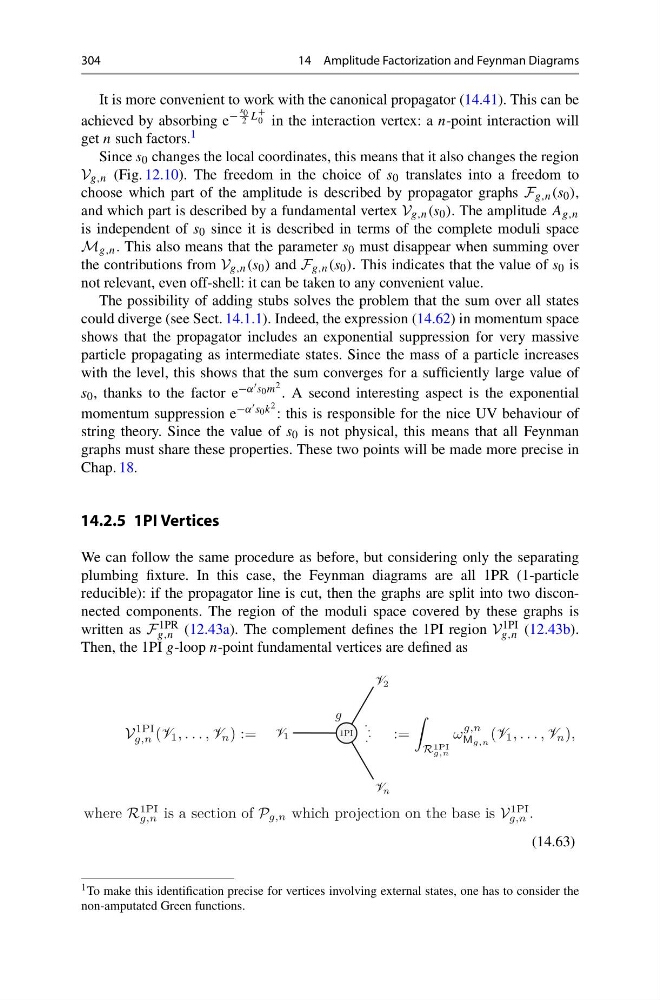
Then, the 1PI g-loop n-point fundamental vertices are defined as
V
1PI
g,n
) :=
:=
R 1PI
g,n
ω
g,n
M g,n
( , . . . , n ),
1
( , . . . , n
1
where R
1PI
g,n is a section of P g,n which projection on the base is V
1PI
g,n .
(14.63)
1 To make this identification precise for vertices involving external states, one has to consider the
non-amputated Green functions.
14 Amplitude Factorization and Feynman Diagrams
It is more convenient to work with the canonical propagator (14.41). This can be
achieved by absorbing e
−
s 0
2 L
+
0 in the interaction vertex: a n-point interaction will
get n such factors. 1
Since s 0 changes the local coordinates, this means that it also changes the region
V g,n (Fig. 12.10). The freedom in the choice of s 0 translates into a freedom to
choose which part of the amplitude is described by propagator graphs F g,n (s 0 ),
and which part is described by a fundamental vertex V g,n (s 0 ). The amplitude A g,n
is independent of s 0 since it is described in terms of the complete moduli space
M g,n . This also means that the parameter s 0 must disappear when summing over
the contributions from V g,n (s 0 ) and F g,n (s 0 ). This indicates that the value of s 0 is
not relevant, even off-shell: it can be taken to any convenient value.
The possibility of adding stubs solves the problem that the sum over all states
could diverge (see Sect. 14.1.1). Indeed, the expression (14.62) in momentum space
shows that the propagator includes an exponential suppression for very massive
particle propagating as intermediate states. Since the mass of a particle increases
with the level, this shows that the sum converges for a sufficiently large value of
s 0 , thanks to the factor e −α s 0 m 2 . A second interesting aspect is the exponential
momentum suppression e −α s 0 k 2 : this is responsible for the nice UV behaviour of
string theory. Since the value of s 0 is not physical, this means that all Feynman
graphs must share these properties. These two points will be made more precise in
Chap. 18.
14.2.5 1PI Vertices
We can follow the same procedure as before, but considering only the separating
plumbing fixture. In this case, the Feynman diagrams are all 1PR (1-particle
reducible): if the propagator line is cut, then the graphs are split into two disconnected components. The region of the moduli space covered by these graphs is
written as F 1PR
g,n (12.43a). The complement defines the 1PI region V 1PI
g,n (12.43b).
Then, the 1PI g-loop n-point fundamental vertices are defined as
V
1PI
g,n
) :=
:=
R 1PI
g,n
ω
g,n
M g,n
( , . . . , n ),
1
( , . . . , n
1
where R
1PI
g,n is a section of P g,n which projection on the base is V
1PI
g,n .
(14.63)
1 To make this identification precise for vertices involving external states, one has to consider the
non-amputated Green functions.