

10.4 Spacetime Action
227
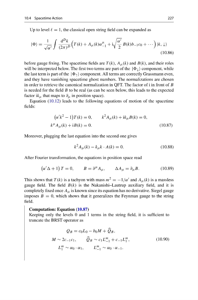
Up to level = 1, the classical open string field can be expanded as
| =
1
√
α
d D k
(2π) D
T (k) + A μ (k)α
μ
−1 + i
α
2
B(k)b −1 c 0 + · · ·
|k, ↓↓
(10.86)
before gauge fixing. The spacetime fields are T (k), A μ (k) and B(k), and their roles
will be interpreted below. The first two terms are part of the | ↓ component, while
the last term is part of the | ↑ component. All terms are correctly Grassmann even,
and they have vanishing spacetime ghost numbers. The normalizations are chosen
in order to retrieve the canonical normalization in QFT. The factor of i in front of B
is needed for the field B to be real (as can be seen below, this leads to the expected
factor ik μ that maps to ∂ μ in position space).
Equation (10.12) leads to the following equations of motion of the spacetime
fields:
α
k
2
− 1
T (k) = 0,
k
2 A μ (k) + ik μ B(k) = 0,
k
μ A μ (k) + iB(k) = 0.
(10.87)
Moreover, plugging the last equation into the second one gives
k
2 A μ (k) − k μ k · A(k) = 0.
(10.88)
After Fourier transformation, the equations in position space read
α
+ 1
T = 0,
B = ∂
μ A μ ,
,A μ = ∂ μ B.
(10.89)
This shows that T (k) is a tachyon with mass m 2 = −1/α and A μ (k) is a massless
gauge field. The field B(k) is the Nakanishi–Lautrup auxiliary field, and it is
completely fixed once A μ is known since its equation has no derivative. Siegel gauge
imposes B = 0, which shows that it generalizes the Feynman gauge to the string
field.
Computation: Equation (10.87)
Keeping only the levels 0 and 1 terms in the string field, it is sufficient to
truncate the BRST operator as
Q B = c 0 L 0 − b 0 M +
Q B ,
M ∼ 2c −1 c 1 ,
Q B ∼ c 1 L
m
−1 + c −1 L
m
1 ,
L
m
1 ∼ α 0 · α 1 ,
L
m
−1 ∼ α 0 · α −1 .
(10.90)
227
Up to level = 1, the classical open string field can be expanded as
| =
1
√
α
d D k
(2π) D
T (k) + A μ (k)α
μ
−1 + i
α
2
B(k)b −1 c 0 + · · ·
|k, ↓↓
(10.86)
before gauge fixing. The spacetime fields are T (k), A μ (k) and B(k), and their roles
will be interpreted below. The first two terms are part of the | ↓ component, while
the last term is part of the | ↑ component. All terms are correctly Grassmann even,
and they have vanishing spacetime ghost numbers. The normalizations are chosen
in order to retrieve the canonical normalization in QFT. The factor of i in front of B
is needed for the field B to be real (as can be seen below, this leads to the expected
factor ik μ that maps to ∂ μ in position space).
Equation (10.12) leads to the following equations of motion of the spacetime
fields:
α
k
2
− 1
T (k) = 0,
k
2 A μ (k) + ik μ B(k) = 0,
k
μ A μ (k) + iB(k) = 0.
(10.87)
Moreover, plugging the last equation into the second one gives
k
2 A μ (k) − k μ k · A(k) = 0.
(10.88)
After Fourier transformation, the equations in position space read
α
+ 1
T = 0,
B = ∂
μ A μ ,
,A μ = ∂ μ B.
(10.89)
This shows that T (k) is a tachyon with mass m 2 = −1/α and A μ (k) is a massless
gauge field. The field B(k) is the Nakanishi–Lautrup auxiliary field, and it is
completely fixed once A μ is known since its equation has no derivative. Siegel gauge
imposes B = 0, which shows that it generalizes the Feynman gauge to the string
field.
Computation: Equation (10.87)
Keeping only the levels 0 and 1 terms in the string field, it is sufficient to
truncate the BRST operator as
Q B = c 0 L 0 − b 0 M +
Q B ,
M ∼ 2c −1 c 1 ,
Q B ∼ c 1 L
m
−1 + c −1 L
m
1 ,
L
m
1 ∼ α 0 · α 1 ,
L
m
−1 ∼ α 0 · α −1 .
(10.90)