

6.4 Operator Formalism and Radial Quantization
119
displayed above. The most striking feature of those theories is that the L 0 operator
is non-diagonalisable (but it can be set in the Jordan normal form).
Remark 6.6 (Fake Identity) Usually, the only primary operator with h = ¯
h = 0 is
the identity 1. While this is always true for unitary theories, there are non-unitary
theories (c ≤ 1 Liouville theory, SLE, loop models) where there is another field
(called the indicator, marking operator, or also fake identity) with h = ¯
h = 0 [1,
5, 16, 19, 27, 31, 33]. The main difference between both fields is that the identity
is a degenerate field (it has a null descendant), whereas the other operator with
h = ¯
h = 0 is not. Such theories will not be considered in this book. Operators
with h = ¯
h = 0 can also be built by combining several CFTs, and they play a very
important role in string theory since they describe on-shell states.
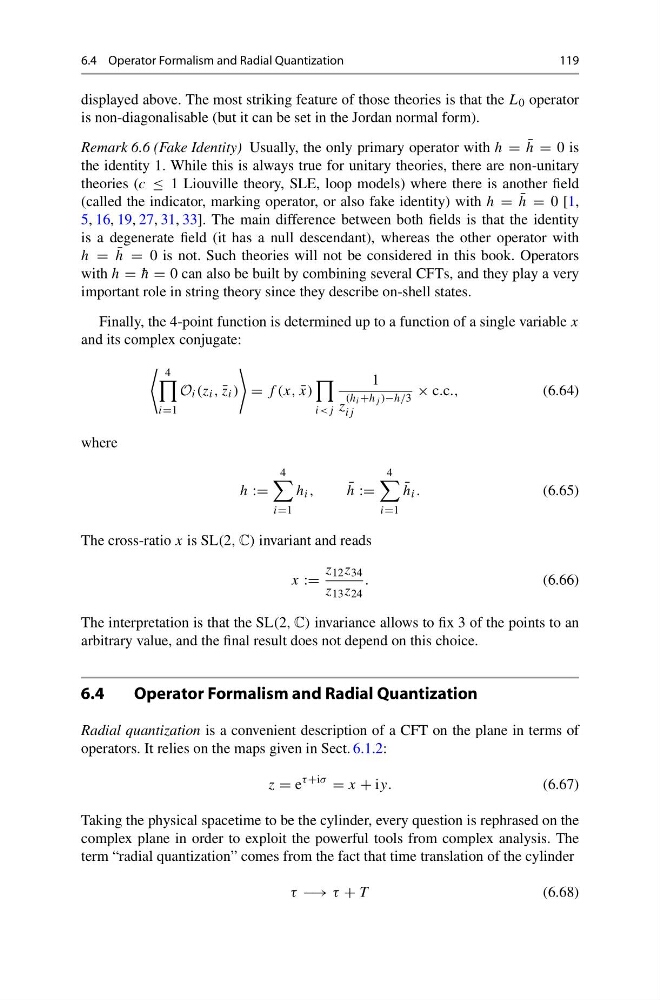
Finally, the 4-point function is determined up to a function of a single variable x
and its complex conjugate:
4
i=1
O i (z i , ¯
z i )
= f (x, ¯
x)
i
z
(h i +h j )−h/3
ij
× c.c.,
(6.64)
where
h :=
4
i=1
h i ,
¯
h :=
4
i=1
¯
h i .
(6.65)
The cross-ratio x is SL(2, C) invariant and reads
x :=
z 12 z 34
z 13 z 24
.
(6.66)
The interpretation is that the SL(2, C) invariance allows to fix 3 of the points to an
arbitrary value, and the final result does not depend on this choice.
6.4
Operator Formalism and Radial Quantization
Radial quantization is a convenient description of a CFT on the plane in terms of
operators. It relies on the maps given in Sect. 6.1.2:
z = e
τ +iσ
= x + iy.
(6.67)
Taking the physical spacetime to be the cylinder, every question is rephrased on the
complex plane in order to exploit the powerful tools from complex analysis. The
term “radial quantization” comes from the fact that time translation of the cylinder
τ −→ τ + T
(6.68)
119
displayed above. The most striking feature of those theories is that the L 0 operator
is non-diagonalisable (but it can be set in the Jordan normal form).
Remark 6.6 (Fake Identity) Usually, the only primary operator with h = ¯
h = 0 is
the identity 1. While this is always true for unitary theories, there are non-unitary
theories (c ≤ 1 Liouville theory, SLE, loop models) where there is another field
(called the indicator, marking operator, or also fake identity) with h = ¯
h = 0 [1,
5, 16, 19, 27, 31, 33]. The main difference between both fields is that the identity
is a degenerate field (it has a null descendant), whereas the other operator with
h = ¯
h = 0 is not. Such theories will not be considered in this book. Operators
with h = ¯
h = 0 can also be built by combining several CFTs, and they play a very
important role in string theory since they describe on-shell states.
Finally, the 4-point function is determined up to a function of a single variable x
and its complex conjugate:
4
i=1
O i (z i , ¯
z i )
= f (x, ¯
x)
i
z
(h i +h j )−h/3
ij
× c.c.,
(6.64)
where
h :=
4
i=1
h i ,
¯
h :=
4
i=1
¯
h i .
(6.65)
The cross-ratio x is SL(2, C) invariant and reads
x :=
z 12 z 34
z 13 z 24
.
(6.66)
The interpretation is that the SL(2, C) invariance allows to fix 3 of the points to an
arbitrary value, and the final result does not depend on this choice.
6.4
Operator Formalism and Radial Quantization
Radial quantization is a convenient description of a CFT on the plane in terms of
operators. It relies on the maps given in Sect. 6.1.2:
z = e
τ +iσ
= x + iy.
(6.67)
Taking the physical spacetime to be the cylinder, every question is rephrased on the
complex plane in order to exploit the powerful tools from complex analysis. The
term “radial quantization” comes from the fact that time translation of the cylinder
τ −→ τ + T
(6.68)