

Me 2 SO
½
¼a∗HU þ b
being [Me 2 SO] the Me 2 SO concentration, in % v/v, HU the
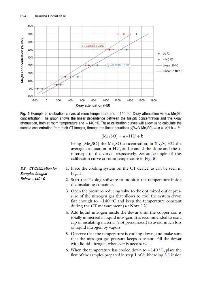
average attenuation in HU, and a and b the slope and the yintercept of the curve, respectively. See an example of this
calibration curve at room temperature in Fig. 5.
3.2 CT Calibration for
Samples Imaged
Below À140
C
1. Place the cooling system on the CT device, as can be seen in
Fig. 1.
2. Start the Picolog software to monitor the temperature inside
the insulating container.
3. Open the pressure-reducing valve to the optimized outlet pressure of the nitrogen gas that allows to cool the system down
fast enough to À140
C and keep the temperature constant
during the CT measurement (see Note 12).
4. Add liquid nitrogen inside the dewar until the copper coil is
totally immersed in liquid nitrogen. It is recommended to use a
cap of insulating material (not pressurized) to avoid much loss
of liquid nitrogen by vapors.
5. Observe that the temperature is cooling down, and make sure
that the nitrogen gas pressure keeps constant. Fill the dewar
with liquid nitrogen whenever is necessary.
6. When the temperature has cooled down to À140
C, place the
first of the samples prepared in step 1 of Subheading 3.1 inside
80%
70%
60%
50%
40%
30%
20%
10%
0%
-10%
-200
0
200
400
600
800
X-ray attenuation (HU)
Me
2 SO concentration (% v/v)
1000
1200
1400
1600
1800
20 ºC
y = 0,0005x + 0,007
y = 0,0004x - 0,033
–140 ºC
Linear 20 ºC
Linear –140 ºC
Fig. 5 Example of calibration curves at room temperature and À140
C: X-ray attenuation versus Me 2 SO
concentration. The graph shows the linear dependence between the Me 2 SO concentration and the X-ray
attenuation, both at room temperature and À140
C. These calibration curves will allow us to calculate the
sample concentration from their CT images, through the linear equations y(%v/v Me 2 SO) ¼ a ∗ x(HU) + b
324
Ariadna Corral et al.
½
¼a∗HU þ b
being [Me 2 SO] the Me 2 SO concentration, in % v/v, HU the
average attenuation in HU, and a and b the slope and the yintercept of the curve, respectively. See an example of this
calibration curve at room temperature in Fig. 5.
3.2 CT Calibration for
Samples Imaged
Below À140
C
1. Place the cooling system on the CT device, as can be seen in
Fig. 1.
2. Start the Picolog software to monitor the temperature inside
the insulating container.
3. Open the pressure-reducing valve to the optimized outlet pressure of the nitrogen gas that allows to cool the system down
fast enough to À140
C and keep the temperature constant
during the CT measurement (see Note 12).
4. Add liquid nitrogen inside the dewar until the copper coil is
totally immersed in liquid nitrogen. It is recommended to use a
cap of insulating material (not pressurized) to avoid much loss
of liquid nitrogen by vapors.
5. Observe that the temperature is cooling down, and make sure
that the nitrogen gas pressure keeps constant. Fill the dewar
with liquid nitrogen whenever is necessary.
6. When the temperature has cooled down to À140
C, place the
first of the samples prepared in step 1 of Subheading 3.1 inside
80%
70%
60%
50%
40%
30%
20%
10%
0%
-10%
-200
0
200
400
600
800
X-ray attenuation (HU)
Me
2 SO concentration (% v/v)
1000
1200
1400
1600
1800
20 ºC
y = 0,0005x + 0,007
y = 0,0004x - 0,033
–140 ºC
Linear 20 ºC
Linear –140 ºC
Fig. 5 Example of calibration curves at room temperature and À140
C: X-ray attenuation versus Me 2 SO
concentration. The graph shows the linear dependence between the Me 2 SO concentration and the X-ray
attenuation, both at room temperature and À140
C. These calibration curves will allow us to calculate the
sample concentration from their CT images, through the linear equations y(%v/v Me 2 SO) ¼ a ∗ x(HU) + b
324
Ariadna Corral et al.