

which can be generalized to
J IIF ¼
ð t
0
minf0, T À f FPD m
i
s ðsÞ, m
i
n ðsÞ
À
Á
g
α i ds:
ð45Þ
This is a generalization of the “two-degree” rule, which is a fixed
limit. This approach accounts for some “accumulation” of the
probability that intracellular ice can form during a protocol. However, it is not as sophisticated as a full IIF model such as one
proposed by Karlsson et al. [123]. Its advantage is in the relative
ease of implementation.
Assembling the solution effects and IIF effects, the total cost of
a cooling approach J cooling can be calculated;
J cooling ¼ J SOL þ kJ IIF ,
ð46Þ
where k is a weighting constant. With this approach, the classic
“inverted U” can be recreated.
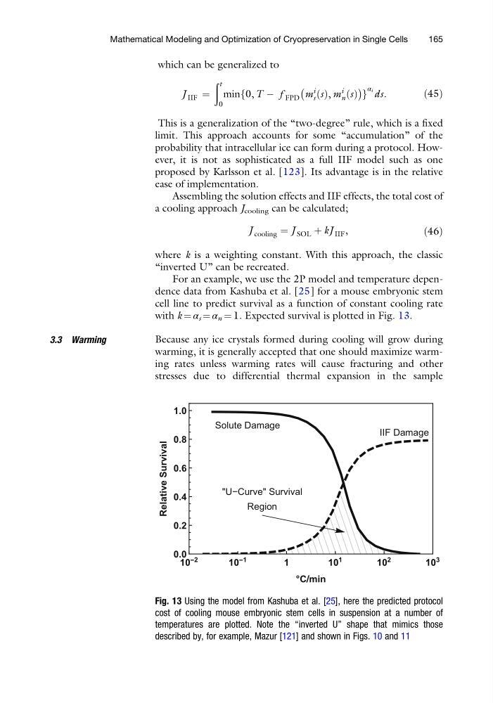
For an example, we use the 2P model and temperature dependence data from Kashuba et al. [25] for a mouse embryonic stem
cell line to predict survival as a function of constant cooling rate
with k ¼ α s ¼ α n ¼ 1. Expected survival is plotted in Fig. 13.
3.3 Warming
Because any ice crystals formed during cooling will grow during
warming, it is generally accepted that one should maximize warming rates unless warming rates will cause fracturing and other
stresses due to differential thermal expansion in the sample
10 −2
10 −1
1
10
1
10
2
10
3
0.0
0.2
0.4
0.6
0.8
1.0
°C/ /min
Relative Survival
Solute Damage
IIF Damage
"U−Curve" Survival
Region
Fig. 13 Using the model from Kashuba et al. [25], here the predicted protocol
cost of cooling mouse embryonic stem cells in suspension at a number of
temperatures are plotted. Note the “inverted U” shape that mimics those
described by, for example, Mazur [121] and shown in Figs. 10 and 11
Mathematical Modeling and Optimization of Cryopreservation in Single Cells
165
J IIF ¼
ð t
0
minf0, T À f FPD m
i
s ðsÞ, m
i
n ðsÞ
À
Á
g
α i ds:
ð45Þ
This is a generalization of the “two-degree” rule, which is a fixed
limit. This approach accounts for some “accumulation” of the
probability that intracellular ice can form during a protocol. However, it is not as sophisticated as a full IIF model such as one
proposed by Karlsson et al. [123]. Its advantage is in the relative
ease of implementation.
Assembling the solution effects and IIF effects, the total cost of
a cooling approach J cooling can be calculated;
J cooling ¼ J SOL þ kJ IIF ,
ð46Þ
where k is a weighting constant. With this approach, the classic
“inverted U” can be recreated.
For an example, we use the 2P model and temperature dependence data from Kashuba et al. [25] for a mouse embryonic stem
cell line to predict survival as a function of constant cooling rate
with k ¼ α s ¼ α n ¼ 1. Expected survival is plotted in Fig. 13.
3.3 Warming
Because any ice crystals formed during cooling will grow during
warming, it is generally accepted that one should maximize warming rates unless warming rates will cause fracturing and other
stresses due to differential thermal expansion in the sample
10 −2
10 −1
1
10
1
10
2
10
3
0.0
0.2
0.4
0.6
0.8
1.0
°C/ /min
Relative Survival
Solute Damage
IIF Damage
"U−Curve" Survival
Region
Fig. 13 Using the model from Kashuba et al. [25], here the predicted protocol
cost of cooling mouse embryonic stem cells in suspension at a number of
temperatures are plotted. Note the “inverted U” shape that mimics those
described by, for example, Mazur [121] and shown in Figs. 10 and 11
Mathematical Modeling and Optimization of Cryopreservation in Single Cells
165