

V ¼
π 0
π
W 0 þ V b :
ð4Þ
Thus, plotting total cell volume against the inverse of extracellular
osmolality yields what is known as a Boyle van ’t Hoff plot (see
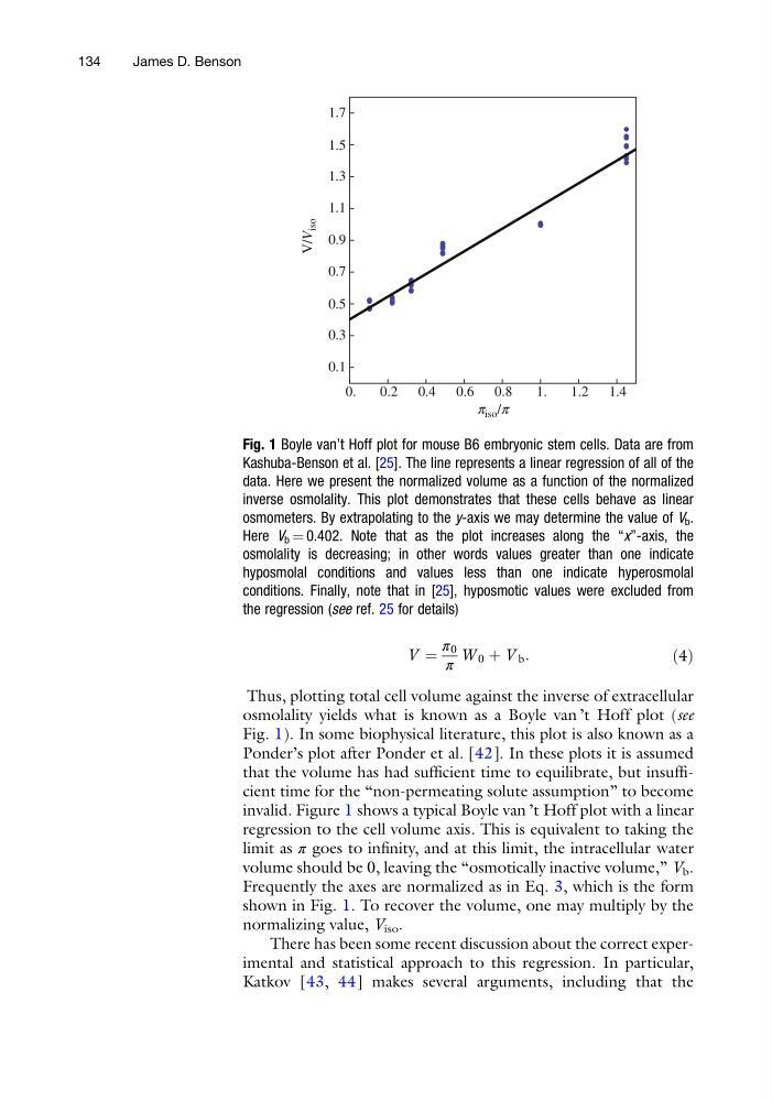
Fig. 1). In some biophysical literature, this plot is also known as a
Ponder’s plot after Ponder et al. [42]. In these plots it is assumed
that the volume has had sufficient time to equilibrate, but insufficient time for the “non-permeating solute assumption” to become
invalid. Figure 1 shows a typical Boyle van ’t Hoff plot with a linear
regression to the cell volume axis. This is equivalent to taking the
limit as π goes to infinity, and at this limit, the intracellular water
volume should be 0, leaving the “osmotically inactive volume,” V b .
Frequently the axes are normalized as in Eq. 3, which is the form
shown in Fig. 1. To recover the volume, one may multiply by the
normalizing value, V iso .
There has been some recent discussion about the correct experimental and statistical approach to this regression. In particular,
Katkov [43, 44] makes several arguments, including that the
0.
0.2 0.4 0.6 0.8
1.
1.2 1.4
0.1
0.3
0.5
0.7
0.9
1.1
1.3
1.5
1.7
p iso /p
V/V
iso
Fig. 1 Boyle van’t Hoff plot for mouse B6 embryonic stem cells. Data are from
Kashuba-Benson et al. [25]. The line represents a linear regression of all of the
data. Here we present the normalized volume as a function of the normalized
inverse osmolality. This plot demonstrates that these cells behave as linear
osmometers. By extrapolating to the y-axis we may determine the value of V b .
Here V b ¼ 0.402. Note that as the plot increases along the “x”-axis, the
osmolality is decreasing; in other words values greater than one indicate
hyposmolal conditions and values less than one indicate hyperosmolal
conditions. Finally, note that in [25], hyposmotic values were excluded from
the regression (see ref. 25 for details)
134
James D. Benson
π 0
π
W 0 þ V b :
ð4Þ
Thus, plotting total cell volume against the inverse of extracellular
osmolality yields what is known as a Boyle van ’t Hoff plot (see
Fig. 1). In some biophysical literature, this plot is also known as a
Ponder’s plot after Ponder et al. [42]. In these plots it is assumed
that the volume has had sufficient time to equilibrate, but insufficient time for the “non-permeating solute assumption” to become
invalid. Figure 1 shows a typical Boyle van ’t Hoff plot with a linear
regression to the cell volume axis. This is equivalent to taking the
limit as π goes to infinity, and at this limit, the intracellular water
volume should be 0, leaving the “osmotically inactive volume,” V b .
Frequently the axes are normalized as in Eq. 3, which is the form
shown in Fig. 1. To recover the volume, one may multiply by the
normalizing value, V iso .
There has been some recent discussion about the correct experimental and statistical approach to this regression. In particular,
Katkov [43, 44] makes several arguments, including that the
0.
0.2 0.4 0.6 0.8
1.
1.2 1.4
0.1
0.3
0.5
0.7
0.9
1.1
1.3
1.5
1.7
p iso /p
V/V
iso
Fig. 1 Boyle van’t Hoff plot for mouse B6 embryonic stem cells. Data are from
Kashuba-Benson et al. [25]. The line represents a linear regression of all of the
data. Here we present the normalized volume as a function of the normalized
inverse osmolality. This plot demonstrates that these cells behave as linear
osmometers. By extrapolating to the y-axis we may determine the value of V b .
Here V b ¼ 0.402. Note that as the plot increases along the “x”-axis, the
osmolality is decreasing; in other words values greater than one indicate
hyposmolal conditions and values less than one indicate hyperosmolal
conditions. Finally, note that in [25], hyposmotic values were excluded from
the regression (see ref. 25 for details)
134
James D. Benson