

2.4 The Static Dielectric Constant
71
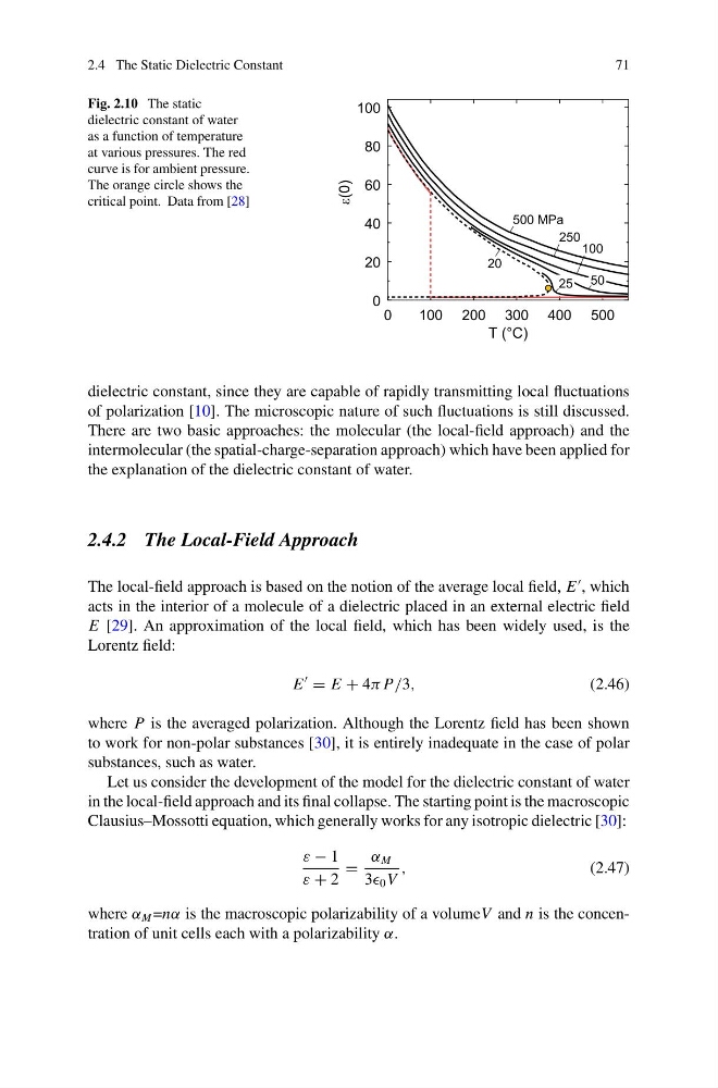
Fig. 2.10 The static
dielectric constant of water
as a function of temperature
at various pressures. The red
curve is for ambient pressure.
The orange circle shows the
critical point. Data from [28]
dielectric constant, since they are capable of rapidly transmitting local fluctuations
of polarization [10]. The microscopic nature of such fluctuations is still discussed.
There are two basic approaches: the molecular (the local-field approach) and the
intermolecular (the spatial-charge-separation approach) which have been applied for
the explanation of the dielectric constant of water.
2.4.2 The Local-Field Approach
The local-field approach is based on the notion of the average local field, E
, which
acts in the interior of a molecule of a dielectric placed in an external electric field
E [29]. An approximation of the local field, which has been widely used, is the
Lorentz field:
E
= E + 4π P/3,
(2.46)
where P is the averaged polarization. Although the Lorentz field has been shown
to work for non-polar substances [30], it is entirely inadequate in the case of polar
substances, such as water.
Let us consider the development of the model for the dielectric constant of water
in the local-field approach and its final collapse. The starting point is the macroscopic
Clausius–Mossotti equation, which generally works for any isotropic dielectric [30]:
ε − 1
ε + 2
=
α M
3 0 V
,
(2.47)
where α M =nα is the macroscopic polarizability of a volumeV and n is the concentration of unit cells each with a polarizability α.
71
Fig. 2.10 The static
dielectric constant of water
as a function of temperature
at various pressures. The red
curve is for ambient pressure.
The orange circle shows the
critical point. Data from [28]
dielectric constant, since they are capable of rapidly transmitting local fluctuations
of polarization [10]. The microscopic nature of such fluctuations is still discussed.
There are two basic approaches: the molecular (the local-field approach) and the
intermolecular (the spatial-charge-separation approach) which have been applied for
the explanation of the dielectric constant of water.
2.4.2 The Local-Field Approach
The local-field approach is based on the notion of the average local field, E
, which
acts in the interior of a molecule of a dielectric placed in an external electric field
E [29]. An approximation of the local field, which has been widely used, is the
Lorentz field:
E
= E + 4π P/3,
(2.46)
where P is the averaged polarization. Although the Lorentz field has been shown
to work for non-polar substances [30], it is entirely inadequate in the case of polar
substances, such as water.
Let us consider the development of the model for the dielectric constant of water
in the local-field approach and its final collapse. The starting point is the macroscopic
Clausius–Mossotti equation, which generally works for any isotropic dielectric [30]:
ε − 1
ε + 2
=
α M
3 0 V
,
(2.47)
where α M =nα is the macroscopic polarizability of a volumeV and n is the concentration of unit cells each with a polarizability α.