

64
2 The Interaction of Electromagnetic Waves with Water
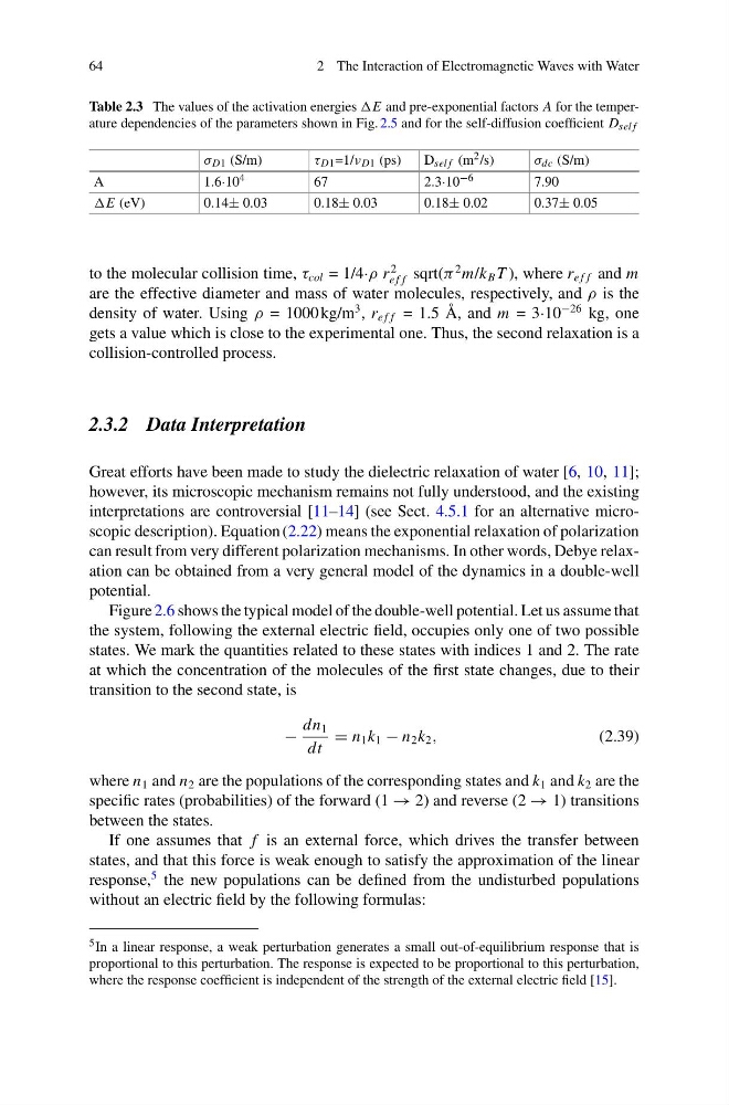
Table 2.3 The values of the activation energies E and pre-exponential factors A for the temperature dependencies of the parameters shown in Fig. 2.5 and for the self-diffusion coefficient D sel f
σ D1 (S/m)
τ D1 =1/ν D1 (ps)
D sel f (m 2 /s)
σ dc (S/m)
A
1.6·10 4
67
2.3·10 −6
7.90
E (eV)
0.14± 0.03
0.18± 0.03
0.18± 0.02
0.37± 0.05
to the molecular collision time, τ col = 1/4·ρ r
2
e f f sqrt(π
2 m/k B T ), where r e f f and m
are the effective diameter and mass of water molecules, respectively, and ρ is the
density of water. Using ρ = 1000 kg/m
3 , r e f f = 1.5 Å, and m = 3·10
−26 kg, one
gets a value which is close to the experimental one. Thus, the second relaxation is a
collision-controlled process.
2.3.2 Data Interpretation
Great efforts have been made to study the dielectric relaxation of water [6, 10, 11];
however, its microscopic mechanism remains not fully understood, and the existing
interpretations are controversial [11–14] (see Sect. 4.5.1 for an alternative microscopic description). Equation (2.22) means the exponential relaxation of polarization
can result from very different polarization mechanisms. In other words, Debye relaxation can be obtained from a very general model of the dynamics in a double-well
potential.
Figure 2.6 shows the typical model of the double-well potential. Let us assume that
the system, following the external electric field, occupies only one of two possible
states. We mark the quantities related to these states with indices 1 and 2. The rate
at which the concentration of the molecules of the first state changes, due to their
transition to the second state, is
−
dn 1
dt
= n 1 k 1 − n 2 k 2 ,
(2.39)
where n 1 and n 2 are the populations of the corresponding states and k 1 and k 2 are the
specific rates (probabilities) of the forward (1 → 2) and reverse (2 → 1) transitions
between the states.
If one assumes that f is an external force, which drives the transfer between
states, and that this force is weak enough to satisfy the approximation of the linear
response,
5 the new populations can be defined from the undisturbed populations
without an electric field by the following formulas:
5 In a linear response, a weak perturbation generates a small out-of-equilibrium response that is
proportional to this perturbation. The response is expected to be proportional to this perturbation,
where the response coefficient is independent of the strength of the external electric field [15].
2 The Interaction of Electromagnetic Waves with Water
Table 2.3 The values of the activation energies E and pre-exponential factors A for the temperature dependencies of the parameters shown in Fig. 2.5 and for the self-diffusion coefficient D sel f
σ D1 (S/m)
τ D1 =1/ν D1 (ps)
D sel f (m 2 /s)
σ dc (S/m)
A
1.6·10 4
67
2.3·10 −6
7.90
E (eV)
0.14± 0.03
0.18± 0.03
0.18± 0.02
0.37± 0.05
to the molecular collision time, τ col = 1/4·ρ r
2
e f f sqrt(π
2 m/k B T ), where r e f f and m
are the effective diameter and mass of water molecules, respectively, and ρ is the
density of water. Using ρ = 1000 kg/m
3 , r e f f = 1.5 Å, and m = 3·10
−26 kg, one
gets a value which is close to the experimental one. Thus, the second relaxation is a
collision-controlled process.
2.3.2 Data Interpretation
Great efforts have been made to study the dielectric relaxation of water [6, 10, 11];
however, its microscopic mechanism remains not fully understood, and the existing
interpretations are controversial [11–14] (see Sect. 4.5.1 for an alternative microscopic description). Equation (2.22) means the exponential relaxation of polarization
can result from very different polarization mechanisms. In other words, Debye relaxation can be obtained from a very general model of the dynamics in a double-well
potential.
Figure 2.6 shows the typical model of the double-well potential. Let us assume that
the system, following the external electric field, occupies only one of two possible
states. We mark the quantities related to these states with indices 1 and 2. The rate
at which the concentration of the molecules of the first state changes, due to their
transition to the second state, is
−
dn 1
dt
= n 1 k 1 − n 2 k 2 ,
(2.39)
where n 1 and n 2 are the populations of the corresponding states and k 1 and k 2 are the
specific rates (probabilities) of the forward (1 → 2) and reverse (2 → 1) transitions
between the states.
If one assumes that f is an external force, which drives the transfer between
states, and that this force is weak enough to satisfy the approximation of the linear
response,
5 the new populations can be defined from the undisturbed populations
without an electric field by the following formulas:
5 In a linear response, a weak perturbation generates a small out-of-equilibrium response that is
proportional to this perturbation. The response is expected to be proportional to this perturbation,
where the response coefficient is independent of the strength of the external electric field [15].