

154
4 The Dielectric Properties and Dynamic Structure of Water and Ice
μ dc =
1
k B T
( f
2
1 + f
2
2 )τ D1
(mγ 1 + Mγ 2 )
2
,
(4.11)
μ ac =
1
k B T
f
2
1 τ D1
m 2 γ
2
1
.
(4.12)
Equation 4.9 is similar to the Debye formula for dielectric relaxation, but it additionally includes the static DC conductivity, σ dc , which is missing in the Debye model
of the orientational polarization of permanent dipolar species. Thus, the ionic model
has a wider range of validity than the Bernal–Fowler model, allowing one to put both
the high- and the low-frequency conductivity on the same footing.
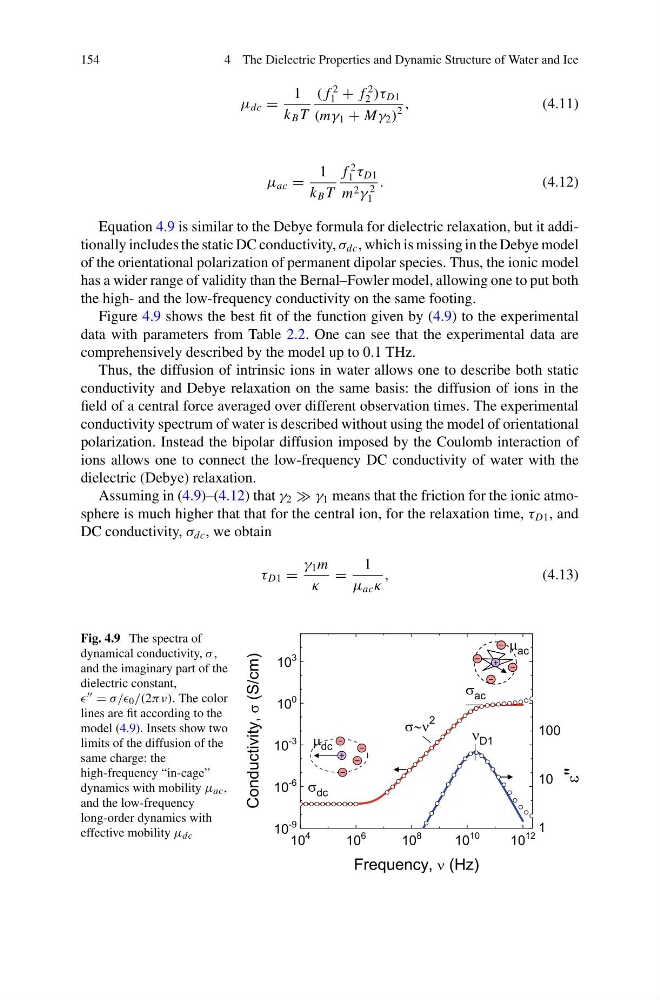
Figure 4.9 shows the best fit of the function given by (4.9) to the experimental
data with parameters from Table 2.2. One can see that the experimental data are
comprehensively described by the model up to 0.1 THz.
Thus, the diffusion of intrinsic ions in water allows one to describe both static
conductivity and Debye relaxation on the same basis: the diffusion of ions in the
field of a central force averaged over different observation times. The experimental
conductivity spectrum of water is described without using the model of orientational
polarization. Instead the bipolar diffusion imposed by the Coulomb interaction of
ions allows one to connect the low-frequency DC conductivity of water with the
dielectric (Debye) relaxation.
Assuming in (4.9)–(4.12) that γ 2 γ 1 means that the friction for the ionic atmosphere is much higher that that for the central ion, for the relaxation time, τ D1 , and
DC conductivity, σ dc , we obtain
τ D1 =
γ 1 m
κ
=
1
μ ac κ
,
(4.13)
Fig. 4.9 The spectra of
dynamical conductivity, σ ,
and the imaginary part of the
dielectric constant,
= σ// 0 /(2πν). The color
lines are fit according to the
model (4.9). Insets show two
limits of the diffusion of the
same charge: the
high-frequency “in-cage”
dynamics with mobility μ ac ,
and the low-frequency
long-order dynamics with
effective mobility μ dc
4 The Dielectric Properties and Dynamic Structure of Water and Ice
μ dc =
1
k B T
( f
2
1 + f
2
2 )τ D1
(mγ 1 + Mγ 2 )
2
,
(4.11)
μ ac =
1
k B T
f
2
1 τ D1
m 2 γ
2
1
.
(4.12)
Equation 4.9 is similar to the Debye formula for dielectric relaxation, but it additionally includes the static DC conductivity, σ dc , which is missing in the Debye model
of the orientational polarization of permanent dipolar species. Thus, the ionic model
has a wider range of validity than the Bernal–Fowler model, allowing one to put both
the high- and the low-frequency conductivity on the same footing.
Figure 4.9 shows the best fit of the function given by (4.9) to the experimental
data with parameters from Table 2.2. One can see that the experimental data are
comprehensively described by the model up to 0.1 THz.
Thus, the diffusion of intrinsic ions in water allows one to describe both static
conductivity and Debye relaxation on the same basis: the diffusion of ions in the
field of a central force averaged over different observation times. The experimental
conductivity spectrum of water is described without using the model of orientational
polarization. Instead the bipolar diffusion imposed by the Coulomb interaction of
ions allows one to connect the low-frequency DC conductivity of water with the
dielectric (Debye) relaxation.
Assuming in (4.9)–(4.12) that γ 2 γ 1 means that the friction for the ionic atmosphere is much higher that that for the central ion, for the relaxation time, τ D1 , and
DC conductivity, σ dc , we obtain
τ D1 =
γ 1 m
κ
=
1
μ ac κ
,
(4.13)
Fig. 4.9 The spectra of
dynamical conductivity, σ ,
and the imaginary part of the
dielectric constant,
= σ// 0 /(2πν). The color
lines are fit according to the
model (4.9). Insets show two
limits of the diffusion of the
same charge: the
high-frequency “in-cage”
dynamics with mobility μ ac ,
and the low-frequency
long-order dynamics with
effective mobility μ dc