

140
4 The Dielectric Properties and Dynamic Structure of Water and Ice
+
+
+
+
II. Secondary relaxation (ν D2 )
1. Ion oscillation
+
3. Diffusion of charge
4. Diffusion of molecule
5. Reconstraction
I. Main (Debye) relaxation (ν D1 )
2. Proton transfer
2'. Separation
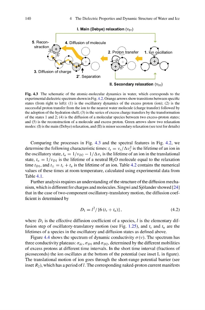
Fig. 4.3 The schematic of the atomic-molecular dynamics in water, which corresponds to the
experimental dielectric spectrum shown in Fig. 4.2. Orange arrows show transitions between specific
states (from right to left): (1) is the oscillatory dynamics of the excess proton (ion); (2) is the
successful proton transfer from the ion to the nearest water molecule (charge transfer) followed by
the adoption of the hydration shell; (3) is the series of excess charge transfers by the transformation
of the states 1 and 2; (4) is the diffusion of a molecular species between two excess-proton states;
and (5) is the reconstruction of a molecule and excess proton. Green arrows show two relaxation
modes: (I) is the main (Debye) relaxation, and (II) is minor secondary relaxation (see text for details)
Comparing the processes in Fig. 4.3 and the spectral features in Fig. 4.2, we
determine the following characteristic times: t s = ν s //ν
2
s is the lifetime of an ion in
the oscillatory state, t u = 1/ν D2 − 1//ν s is the lifetime of an ion in the translational
state, t w = 1/ν D1 is the lifetime of a neutral H 2 O molecule equal to the relaxation
time t D1 , and t ± = t s + t u is the lifetime of an ion. Table 4.2 contains the numerical
values of these times at room temperature, calculated using experimental data from
Table 4.1.
Further analysis requires an understanding of the structure of the diffusion mechanism, which is different for charges and molecules. Singwi and Sjölander showed [24]
that in the case of two-component oscillatory-translatory motion, the diffusion coefficient is determined by
D 1 = l
2
/ [6 (t s + t u )] ,
(4.2)
where D 1 is the effective diffusion coefficient of a species, l is the elementary diffusion step of oscillatory-translatory motion (see Fig. 1.25), and t s and t u are the
lifetimes of a species in the oscillatory and diffusion states as defined above.
Figure 4.4 shows the spectrum of dynamic conductivity σ (ν). The spectrum has
three conductivity plateaus: σ dc , σ D1 and σ D2 , determined by the different mobilities
of excess protons at different time intervals. In the short time interval (fractions of
picoseconds) the ion oscillates at the bottom of the potential (see inset L in figure).
The translational motion of ion goes through the short-range potential barrier (see
inset R 2 ), which has a period of l. The corresponding naked-proton current manifests
4 The Dielectric Properties and Dynamic Structure of Water and Ice
+
+
+
+
II. Secondary relaxation (ν D2 )
1. Ion oscillation
+
3. Diffusion of charge
4. Diffusion of molecule
5. Reconstraction
I. Main (Debye) relaxation (ν D1 )
2. Proton transfer
2'. Separation
Fig. 4.3 The schematic of the atomic-molecular dynamics in water, which corresponds to the
experimental dielectric spectrum shown in Fig. 4.2. Orange arrows show transitions between specific
states (from right to left): (1) is the oscillatory dynamics of the excess proton (ion); (2) is the
successful proton transfer from the ion to the nearest water molecule (charge transfer) followed by
the adoption of the hydration shell; (3) is the series of excess charge transfers by the transformation
of the states 1 and 2; (4) is the diffusion of a molecular species between two excess-proton states;
and (5) is the reconstruction of a molecule and excess proton. Green arrows show two relaxation
modes: (I) is the main (Debye) relaxation, and (II) is minor secondary relaxation (see text for details)
Comparing the processes in Fig. 4.3 and the spectral features in Fig. 4.2, we
determine the following characteristic times: t s = ν s //ν
2
s is the lifetime of an ion in
the oscillatory state, t u = 1/ν D2 − 1//ν s is the lifetime of an ion in the translational
state, t w = 1/ν D1 is the lifetime of a neutral H 2 O molecule equal to the relaxation
time t D1 , and t ± = t s + t u is the lifetime of an ion. Table 4.2 contains the numerical
values of these times at room temperature, calculated using experimental data from
Table 4.1.
Further analysis requires an understanding of the structure of the diffusion mechanism, which is different for charges and molecules. Singwi and Sjölander showed [24]
that in the case of two-component oscillatory-translatory motion, the diffusion coefficient is determined by
D 1 = l
2
/ [6 (t s + t u )] ,
(4.2)
where D 1 is the effective diffusion coefficient of a species, l is the elementary diffusion step of oscillatory-translatory motion (see Fig. 1.25), and t s and t u are the
lifetimes of a species in the oscillatory and diffusion states as defined above.
Figure 4.4 shows the spectrum of dynamic conductivity σ (ν). The spectrum has
three conductivity plateaus: σ dc , σ D1 and σ D2 , determined by the different mobilities
of excess protons at different time intervals. In the short time interval (fractions of
picoseconds) the ion oscillates at the bottom of the potential (see inset L in figure).
The translational motion of ion goes through the short-range potential barrier (see
inset R 2 ), which has a period of l. The corresponding naked-proton current manifests