

3.4 Similarities Between Water and Ice
119
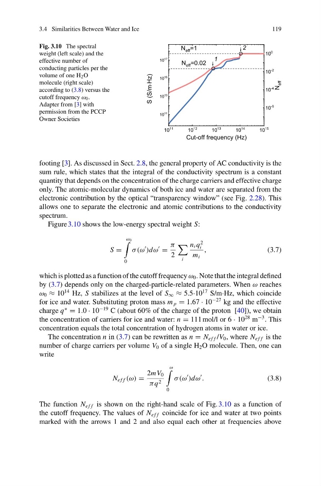
Fig. 3.10 The spectral
weight (left scale) and the
effective number of
conducting particles per the
volume of one H 2 O
molecule (right scale)
according to (3.8) versus the
cutoff frequency ω 0 .
Adapter from [3] with
permission from the PCCP
Owner Societies
footing [3]. As discussed in Sect. 2.8, the general property of AC conductivity is the
sum rule, which states that the integral of the conductivity spectrum is a constant
quantity that depends on the concentration of the charge carriers and effective charge
only. The atomic-molecular dynamics of both ice and water are separated from the
electronic contribution by the optical “transparency window” (see Fig. 2.28). This
allows one to separate the electronic and atomic contributions to the conductivity
spectrum.
Figure 3.10 shows the low-energy spectral weight S:
S =
ω 0
0
σ (ω
)dω
=
π
2
i
n i q
2
i
m i
,
(3.7)
which is plotted as a function of the cutoff frequency ω 0 . Note that the integral defined
by (3.7) depends only on the charged-particle-related parameters. When ω reaches
ω 0 ≈ 10
14 Hz, S stabilizes at the level of S ∞ ≈ 5.5·10
17 S/m·Hz, which coincide
for ice and water. Substituting proton mass m p = 1.67 · 10
−27 kg and the effective
charge q
∗
= 1.0 · 10
−19 C (about 60% of the charge of the proton [40]), we obtain
the concentration of carriers for ice and water: n = 111 mol/l or 6 · 10
28 m
−3 . This
concentration equals the total concentration of hydrogen atoms in water or ice.
The concentration n in (3.7) can be rewritten as n = N e f f /V 0 , where N e f f is the
number of charge carriers per volume V 0 of a single H 2 O molecule. Then, one can
write
N e f f (ω) =
2mV 0
πq 2
ω
0
σ (ω
)dω
.
(3.8)
The function N e f f is shown on the right-hand scale of Fig. 3.10 as a function of
the cutoff frequency. The values of N e f f coincide for ice and water at two points
marked with the arrows 1 and 2 and also equal each other at frequencies above
119
Fig. 3.10 The spectral
weight (left scale) and the
effective number of
conducting particles per the
volume of one H 2 O
molecule (right scale)
according to (3.8) versus the
cutoff frequency ω 0 .
Adapter from [3] with
permission from the PCCP
Owner Societies
footing [3]. As discussed in Sect. 2.8, the general property of AC conductivity is the
sum rule, which states that the integral of the conductivity spectrum is a constant
quantity that depends on the concentration of the charge carriers and effective charge
only. The atomic-molecular dynamics of both ice and water are separated from the
electronic contribution by the optical “transparency window” (see Fig. 2.28). This
allows one to separate the electronic and atomic contributions to the conductivity
spectrum.
Figure 3.10 shows the low-energy spectral weight S:
S =
ω 0
0
σ (ω
)dω
=
π
2
i
n i q
2
i
m i
,
(3.7)
which is plotted as a function of the cutoff frequency ω 0 . Note that the integral defined
by (3.7) depends only on the charged-particle-related parameters. When ω reaches
ω 0 ≈ 10
14 Hz, S stabilizes at the level of S ∞ ≈ 5.5·10
17 S/m·Hz, which coincide
for ice and water. Substituting proton mass m p = 1.67 · 10
−27 kg and the effective
charge q
∗
= 1.0 · 10
−19 C (about 60% of the charge of the proton [40]), we obtain
the concentration of carriers for ice and water: n = 111 mol/l or 6 · 10
28 m
−3 . This
concentration equals the total concentration of hydrogen atoms in water or ice.
The concentration n in (3.7) can be rewritten as n = N e f f /V 0 , where N e f f is the
number of charge carriers per volume V 0 of a single H 2 O molecule. Then, one can
write
N e f f (ω) =
2mV 0
πq 2
ω
0
σ (ω
)dω
.
(3.8)
The function N e f f is shown on the right-hand scale of Fig. 3.10 as a function of
the cutoff frequency. The values of N e f f coincide for ice and water at two points
marked with the arrows 1 and 2 and also equal each other at frequencies above