

2.8 The Conductivity Sum Rule
99
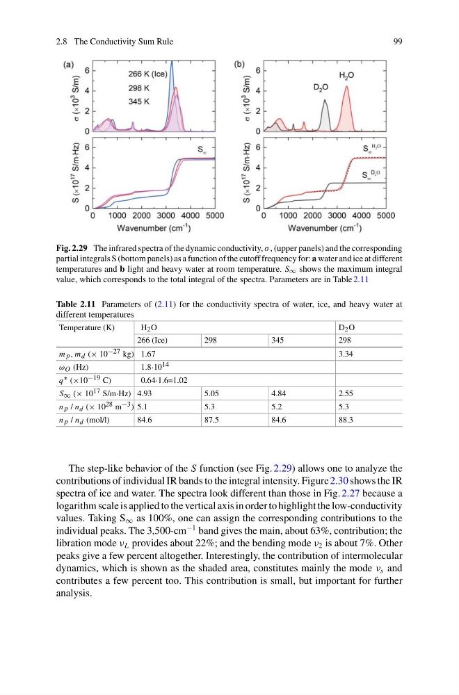
Fig. 2.29 The infrared spectra of the dynamic conductivity, σ , (upper panels) and the corresponding
partial integrals S (bottom panels) as a function of the cutoff frequency for: a water and ice at different
temperatures and b light and heavy water at room temperature. S ∞ shows the maximum integral
value, which corresponds to the total integral of the spectra. Parameters are in Table 2.11
Table 2.11 Parameters of (2.11) for the conductivity spectra of water, ice, and heavy water at
different temperatures
Temperature (K)
H 2 O
D 2 O
266 (Ice)
298
345
298
m p , m d (× 10 −27 kg) 1.67
3.34
ω O (Hz)
1.8·10 14
q ∗ (×10 −19 C)
0.64·1.6=1.02
S ∞ (× 10 17 S/m·Hz) 4.93
5.05
4.84
2.55
n p / n d (× 10 28 m −3 ) 5.1
5.3
5.2
5.3
n p / n d (mol/l)
84.6
87.5
84.6
88.3
The step-like behavior of the S function (see Fig. 2.29) allows one to analyze the
contributions of individual IR bands to the integral intensity. Figure 2.30 shows the IR
spectra of ice and water. The spectra look different than those in Fig. 2.27 because a
logarithm scale is applied to the vertical axis in order to highlight the low-conductivity
values. Taking S ∞ as 100%, one can assign the corresponding contributions to the
individual peaks. The 3,500-cm
−1 band gives the main, about 63%, contribution; the
libration mode ν L provides about 22%; and the bending mode ν 2 is about 7%. Other
peaks give a few percent altogether. Interestingly, the contribution of intermolecular
dynamics, which is shown as the shaded area, constitutes mainly the mode ν s and
contributes a few percent too. This contribution is small, but important for further
analysis.
99
Fig. 2.29 The infrared spectra of the dynamic conductivity, σ , (upper panels) and the corresponding
partial integrals S (bottom panels) as a function of the cutoff frequency for: a water and ice at different
temperatures and b light and heavy water at room temperature. S ∞ shows the maximum integral
value, which corresponds to the total integral of the spectra. Parameters are in Table 2.11
Table 2.11 Parameters of (2.11) for the conductivity spectra of water, ice, and heavy water at
different temperatures
Temperature (K)
H 2 O
D 2 O
266 (Ice)
298
345
298
m p , m d (× 10 −27 kg) 1.67
3.34
ω O (Hz)
1.8·10 14
q ∗ (×10 −19 C)
0.64·1.6=1.02
S ∞ (× 10 17 S/m·Hz) 4.93
5.05
4.84
2.55
n p / n d (× 10 28 m −3 ) 5.1
5.3
5.2
5.3
n p / n d (mol/l)
84.6
87.5
84.6
88.3
The step-like behavior of the S function (see Fig. 2.29) allows one to analyze the
contributions of individual IR bands to the integral intensity. Figure 2.30 shows the IR
spectra of ice and water. The spectra look different than those in Fig. 2.27 because a
logarithm scale is applied to the vertical axis in order to highlight the low-conductivity
values. Taking S ∞ as 100%, one can assign the corresponding contributions to the
individual peaks. The 3,500-cm
−1 band gives the main, about 63%, contribution; the
libration mode ν L provides about 22%; and the bending mode ν 2 is about 7%. Other
peaks give a few percent altogether. Interestingly, the contribution of intermolecular
dynamics, which is shown as the shaded area, constitutes mainly the mode ν s and
contributes a few percent too. This contribution is small, but important for further
analysis.