

96
2 The Interaction of Electromagnetic Waves with Water
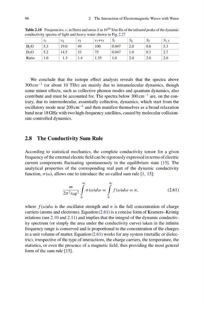
Table 2.10 Frequencies, ν, in Hertz and areas S in 10 16 S/m·Hz of the infrared peaks of the dynamic
conductivity spectra of light and heavy water shown in Fig. 2.27
ν s
ν L
ν 2
ν 1 +ν 3
S s
S L
S 2
S 1,3
H 2 O
5.3
19.0
49
100
0.047
2.0
0.6
5.3
D 2 O
5.2
14.5
33
75
0.047
1.0
0.3
2.7
Ratio
1.0
1.3
1.4
1.35
1.0
2.0
2.0
2.0
We conclude that the isotope effect analysis reveals that the spectra above
300 cm
−1 (or about 10 THz) are mainly due to intramolecular dynamics, though
some minor effects, such as collective phonon modes and quantum dynamics, also
contribute and must be accounted for. The spectra below 300 cm
−1 are, on the contrary, due to intermolecular, essentially collective, dynamics, which start from the
oscillatory mode near 200 cm
−1 and then manifest themselves as a broad relaxation
band near 18 GHz with two high-frequency satellites, caused by molecular collisionrate-controlled dynamics.
2.8 The Conductivity Sum Rule
According to statistical mechanics, the complete conductivity tensor for a given
frequency of the external electric field can be rigorously expressed in terms of electric
current components fluctuating spontaneously in the equilibrium state [15]. The
analytical properties of the corresponding real part of the dynamic conductivity
function, σ (ω), allows one to introduce the so-called sum rule [1, 15]:
m
2π 2 ε 0 q 2
∞
0
σ (ω)dω =
∞
0
f (ω)dω = n,
(2.61)
where f (ω)dω is the oscillator strength and n is the full concentration of charge
carriers (atoms and electrons). Equation (2.61) is a concise form of Kramers–Kronig
relations (see 2.10 and 2.11) and implies that the integral of the dynamic conductivity spectrum (or simply the area under the conductivity curve) taken in the infinite
frequency range is conserved and is proportional to the concentration of the charges
in a unit volume of matter. Equation (2.61) works for any system (metallic or dielectric), irrespective of the type of interactions, the charge carriers, the temperature, the
statistics, or even the presence of a magnetic field, thus providing the most general
form of the sum rule [15].
2 The Interaction of Electromagnetic Waves with Water
Table 2.10 Frequencies, ν, in Hertz and areas S in 10 16 S/m·Hz of the infrared peaks of the dynamic
conductivity spectra of light and heavy water shown in Fig. 2.27
ν s
ν L
ν 2
ν 1 +ν 3
S s
S L
S 2
S 1,3
H 2 O
5.3
19.0
49
100
0.047
2.0
0.6
5.3
D 2 O
5.2
14.5
33
75
0.047
1.0
0.3
2.7
Ratio
1.0
1.3
1.4
1.35
1.0
2.0
2.0
2.0
We conclude that the isotope effect analysis reveals that the spectra above
300 cm
−1 (or about 10 THz) are mainly due to intramolecular dynamics, though
some minor effects, such as collective phonon modes and quantum dynamics, also
contribute and must be accounted for. The spectra below 300 cm
−1 are, on the contrary, due to intermolecular, essentially collective, dynamics, which start from the
oscillatory mode near 200 cm
−1 and then manifest themselves as a broad relaxation
band near 18 GHz with two high-frequency satellites, caused by molecular collisionrate-controlled dynamics.
2.8 The Conductivity Sum Rule
According to statistical mechanics, the complete conductivity tensor for a given
frequency of the external electric field can be rigorously expressed in terms of electric
current components fluctuating spontaneously in the equilibrium state [15]. The
analytical properties of the corresponding real part of the dynamic conductivity
function, σ (ω), allows one to introduce the so-called sum rule [1, 15]:
m
2π 2 ε 0 q 2
∞
0
σ (ω)dω =
∞
0
f (ω)dω = n,
(2.61)
where f (ω)dω is the oscillator strength and n is the full concentration of charge
carriers (atoms and electrons). Equation (2.61) is a concise form of Kramers–Kronig
relations (see 2.10 and 2.11) and implies that the integral of the dynamic conductivity spectrum (or simply the area under the conductivity curve) taken in the infinite
frequency range is conserved and is proportional to the concentration of the charges
in a unit volume of matter. Equation (2.61) works for any system (metallic or dielectric), irrespective of the type of interactions, the charge carriers, the temperature, the
statistics, or even the presence of a magnetic field, thus providing the most general
form of the sum rule [15].