

z 1
z 2
z 3
z 4
z 5
z 6
z 7
z 8
z 9
58
Biomedical Signal and Image Processing
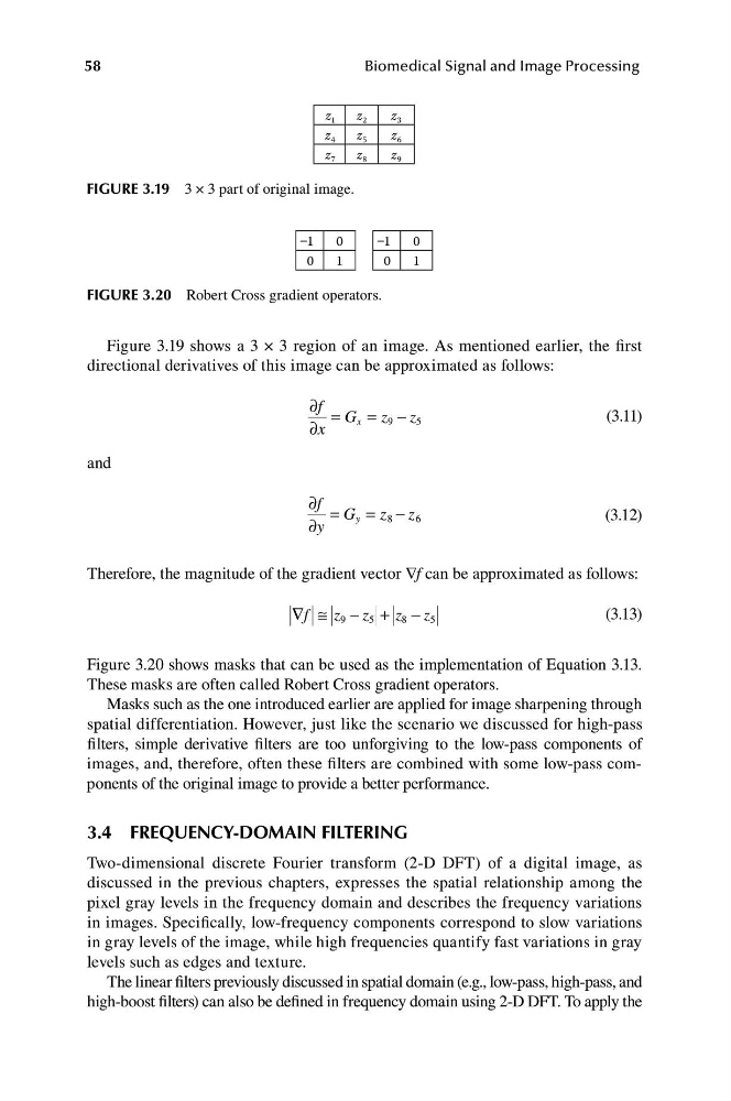
FIGURE 3.19 3 × 3 part of original image.
–1
0
0
1
–1
0
0
1
FIGURE 3.20 Robert Cross gradient operators.
Figure 3.19 shows a 3 × 3 region of an image. As mentioned earlier, the first
directional derivatives of this image can be approximated as follows:
∂f = G
∂
x = z 9 − z
x
5
(3.11)
and
∂f = G y = z
∂y
8 − z 6
(3.12)
Therefore, the magnitude of the gradient vector ∇f can be approximated as follows:
∇ ≅
f
z 9 − z
(3
5 + z 8 − z 5
.13)
Figure 3.20 shows masks that can be used as the implementation of Equation 3.13.
These masks are often called Robert Cross gradient operators.
Masks such as the one introduced earlier are applied for image sharpening through
spatial differentiation. However, just like the scenario we discussed for high-pass
filters, simple derivative filters are too unforgiving to the low-pass components of
images, and, therefore, often these filters are combined with some low-pass components of the original image to provide a better performance.
3.4 FREQUENCY-DOMAIN FILTERING
Two-dimensional discrete Fourier transform (2-D DFT) of a digital image, as
discussed in the previous chapters, expresses the spatial relationship among the
pixel gray levels in the frequency domain and describes the frequency variations
in images. Specifically, low-frequency components correspond to slow variations
in gray levels of the image, while high frequencies quantify fast variations in gray
levels such as edges and texture.
The linear filters previously discussed in spatial domain (e.g., low-pass, high-pass, and
high-boost filters) can also be defined in frequency domain using 2-D DFT. To apply the
z 2
z 3
z 4
z 5
z 6
z 7
z 8
z 9
58
Biomedical Signal and Image Processing
FIGURE 3.19 3 × 3 part of original image.
–1
0
0
1
–1
0
0
1
FIGURE 3.20 Robert Cross gradient operators.
Figure 3.19 shows a 3 × 3 region of an image. As mentioned earlier, the first
directional derivatives of this image can be approximated as follows:
∂f = G
∂
x = z 9 − z
x
5
(3.11)
and
∂f = G y = z
∂y
8 − z 6
(3.12)
Therefore, the magnitude of the gradient vector ∇f can be approximated as follows:
∇ ≅
f
z 9 − z
(3
5 + z 8 − z 5
.13)
Figure 3.20 shows masks that can be used as the implementation of Equation 3.13.
These masks are often called Robert Cross gradient operators.
Masks such as the one introduced earlier are applied for image sharpening through
spatial differentiation. However, just like the scenario we discussed for high-pass
filters, simple derivative filters are too unforgiving to the low-pass components of
images, and, therefore, often these filters are combined with some low-pass components of the original image to provide a better performance.
3.4 FREQUENCY-DOMAIN FILTERING
Two-dimensional discrete Fourier transform (2-D DFT) of a digital image, as
discussed in the previous chapters, expresses the spatial relationship among the
pixel gray levels in the frequency domain and describes the frequency variations
in images. Specifically, low-frequency components correspond to slow variations
in gray levels of the image, while high frequencies quantify fast variations in gray
levels such as edges and texture.
The linear filters previously discussed in spatial domain (e.g., low-pass, high-pass, and
high-boost filters) can also be defined in frequency domain using 2-D DFT. To apply the