

1
1
1
(1/9)*
1
1
1
1
1
1
1
2
1
(1/16)*
2
4
2
1
2
1
(a)
(b)
49
Image Filtering, Enhancement, and Restoration
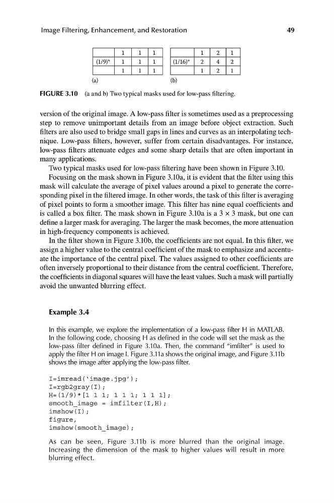
FIGURE 3.10 (a and b) Two typical masks used for low-pass filtering.
version of the original image. A low-pass filter is sometimes used as a preprocessing
step to remove unimportant details from an image before object extraction. Such
filters are also used to bridge small gaps in lines and curves as an interpolating technique. Low-pass filters, however, suffer from certain disadvantages. For instance,
low-pass filters attenuate edges and some sharp details that are often important in
many applications.
Two typical masks used for low-pass filtering have been shown in Figure 3.10.
Focusing on the mask shown in Figure 3.10a, it is evident that the filter using this
mask will calculate the average of pixel values around a pixel to generate the corresponding pixel in the filtered image. In other words, the task of this filter is averaging
of pixel points to form a smoother image. This filter has nine equal coefficients and
is called a box filter. The mask shown in Figure 3.10a is a 3 × 3 mask, but one can
define a larger mask for averaging. The larger the mask becomes, the more attenuation
in high-frequency components is achieved.
In the filter shown in Figure 3.10b, the coefficients are not equal. In this filter, we
assign a higher value to the central coefficient of the mask to emphasize and accentuate the importance of the central pixel. The values assigned to other coefficients are
often inversely proportional to their distance from the central coefficient. Therefore,
the coefficients in diagonal squares will have the least values. Such a mask will partially
avoid the unwanted blurring effect.
Example 3.4
In this example, we explore the implementation of a low-pass filter H in MATLAB.
In the following code, choosing H as defined in the code will set the mask as the
low-pass filter defined in Figure 3.10a. Then, the command “imfilter” is used to
apply the filter H on image I. Figure 3.11a shows the original image, and Figure 3.11b
shows the image after applying the low-pass filter.
I=imread(‘image.jpg’);
I=rgb2gray(I);
H=(1/9)*[1 1 1; 1 1 1; 1 1 1];
smooth_image = imfilter(I,H);
imshow(I);
figure,
imshow(smooth_image);
As can be seen, Figure 3.11b is more blurred than the original image.
Increasing the dimension of the mask to higher values will result in more
blurring effect.
1
1
(1/9)*
1
1
1
1
1
1
1
2
1
(1/16)*
2
4
2
1
2
1
(a)
(b)
49
Image Filtering, Enhancement, and Restoration
FIGURE 3.10 (a and b) Two typical masks used for low-pass filtering.
version of the original image. A low-pass filter is sometimes used as a preprocessing
step to remove unimportant details from an image before object extraction. Such
filters are also used to bridge small gaps in lines and curves as an interpolating technique. Low-pass filters, however, suffer from certain disadvantages. For instance,
low-pass filters attenuate edges and some sharp details that are often important in
many applications.
Two typical masks used for low-pass filtering have been shown in Figure 3.10.
Focusing on the mask shown in Figure 3.10a, it is evident that the filter using this
mask will calculate the average of pixel values around a pixel to generate the corresponding pixel in the filtered image. In other words, the task of this filter is averaging
of pixel points to form a smoother image. This filter has nine equal coefficients and
is called a box filter. The mask shown in Figure 3.10a is a 3 × 3 mask, but one can
define a larger mask for averaging. The larger the mask becomes, the more attenuation
in high-frequency components is achieved.
In the filter shown in Figure 3.10b, the coefficients are not equal. In this filter, we
assign a higher value to the central coefficient of the mask to emphasize and accentuate the importance of the central pixel. The values assigned to other coefficients are
often inversely proportional to their distance from the central coefficient. Therefore,
the coefficients in diagonal squares will have the least values. Such a mask will partially
avoid the unwanted blurring effect.
Example 3.4
In this example, we explore the implementation of a low-pass filter H in MATLAB.
In the following code, choosing H as defined in the code will set the mask as the
low-pass filter defined in Figure 3.10a. Then, the command “imfilter” is used to
apply the filter H on image I. Figure 3.11a shows the original image, and Figure 3.11b
shows the image after applying the low-pass filter.
I=imread(‘image.jpg’);
I=rgb2gray(I);
H=(1/9)*[1 1 1; 1 1 1; 1 1 1];
smooth_image = imfilter(I,H);
imshow(I);
figure,
imshow(smooth_image);
As can be seen, Figure 3.11b is more blurred than the original image.
Increasing the dimension of the mask to higher values will result in more
blurring effect.