

RA
RA
SVC
SVC
RPA
RPA
LA
LA
R
R
(a)
(b)
42
Biomedical Signal and Image Processing
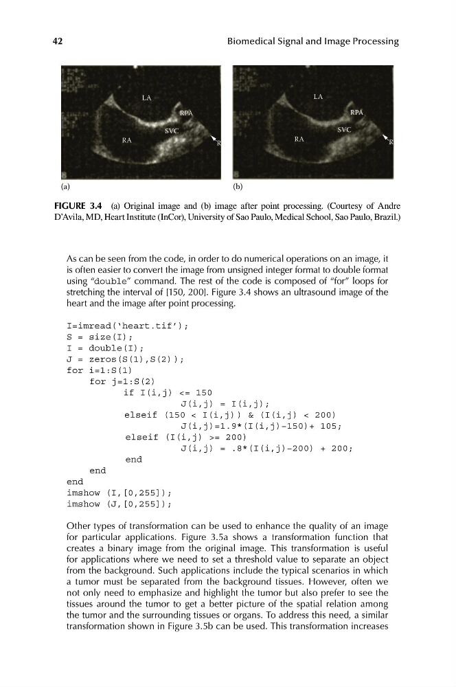
FIGURE 3.4 (a) Original image and (b) image after point processing. (Courtesy of Andre
D’Avila, MD, Heart Institute (InCor), University of Sao Paulo, Medical School, Sao Paulo, Brazil.)
As can be seen from the code, in order to do numerical operations on an image, it
is often easier to convert the image from unsigned integer format to double format
using “double” command. The rest of the code is composed of “for” loops for
stretching the interval of [150, 200]. Figure 3.4 shows an ultrasound image of the
heart and the image after point processing.
I=imread(‘heart.tif’);
S = size(I);
I = double(I);
J = zeros(S(1),S(2) );
for i=1:S(1)
for j=1:S(2)
if I(i,j) <= 150
J(i,j) = I(i,j);
elseif (150 < I(i,j) ) & (I(i,j) < 200)
J(i,j)=1.9*(I(i,j)−150)+ 105;
elseif (I(i,j) >= 200)
J(i,j) = .8*(I(i,j)−200) + 200;
end
end
end
imshow (I,[0,255]);
imshow (J,[0,255]);
Other types of transformation can be used to enhance the quality of an image
for particular applications. Figure 3.5a shows a transformation function that
creates a binary image from the original image. This transformation is useful
for applications where we need to set a threshold value to separate an object
from the background. Such applications include the typical scenarios in which
a tumor must be separated from the background tissues. However, often we
not only need to emphasize and highlight the tumor but also prefer to see the
tissues around the tumor to get a better picture of the spatial relation among
the tumor and the surrounding tissues or organs. To address this need, a similar
transformation shown in Figure 3.5b can be used. This transformation increases
RA
SVC
SVC
RPA
RPA
LA
LA
R
R
(a)
(b)
42
Biomedical Signal and Image Processing
FIGURE 3.4 (a) Original image and (b) image after point processing. (Courtesy of Andre
D’Avila, MD, Heart Institute (InCor), University of Sao Paulo, Medical School, Sao Paulo, Brazil.)
As can be seen from the code, in order to do numerical operations on an image, it
is often easier to convert the image from unsigned integer format to double format
using “double” command. The rest of the code is composed of “for” loops for
stretching the interval of [150, 200]. Figure 3.4 shows an ultrasound image of the
heart and the image after point processing.
I=imread(‘heart.tif’);
S = size(I);
I = double(I);
J = zeros(S(1),S(2) );
for i=1:S(1)
for j=1:S(2)
if I(i,j) <= 150
J(i,j) = I(i,j);
elseif (150 < I(i,j) ) & (I(i,j) < 200)
J(i,j)=1.9*(I(i,j)−150)+ 105;
elseif (I(i,j) >= 200)
J(i,j) = .8*(I(i,j)−200) + 200;
end
end
end
imshow (I,[0,255]);
imshow (J,[0,255]);
Other types of transformation can be used to enhance the quality of an image
for particular applications. Figure 3.5a shows a transformation function that
creates a binary image from the original image. This transformation is useful
for applications where we need to set a threshold value to separate an object
from the background. Such applications include the typical scenarios in which
a tumor must be separated from the background tissues. However, often we
not only need to emphasize and highlight the tumor but also prefer to see the
tissues around the tumor to get a better picture of the spatial relation among
the tumor and the surrounding tissues or organs. To address this need, a similar
transformation shown in Figure 3.5b can be used. This transformation increases