

37
Fourier Transform
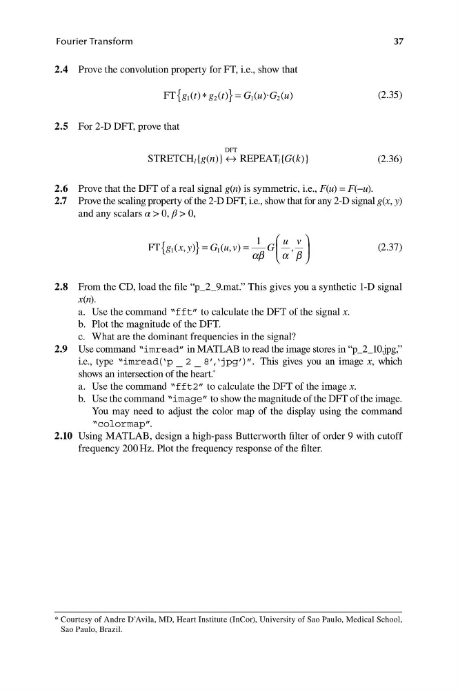
2.4 Prove the convolution property for FT, i.e., show that
FT { g t
1 ( )∗ g 2 ( )
t } = G 1 (u) . G 2 ( )
u
(2.35)
2.5 For 2-D DFT, prove that
DFT
STRETCH l { g n
( )} ↔ REPEAT l { G( k )}
(2.36)
2.6 Prove that the DFT of a real signal g(n) is symmetric, i.e., F(u) = F(−u).
2.7 P rove the scaling property of the 2-D DFT, i.e., show that for any 2-D signal g(x, y)
and any scalars α > 0, β > 0,
{
}
1 ⎛ u v ⎞
FT g x
1 ( , y ) = G 1 (u, v) =
G ⎜ , ⎟
(2.37)
ab ⎝ a b ⎠
2.8 Fro m the CD, load the file “p_2_9.mat.” This gives you a synthetic 1-D signal
x(n).
a. Use the command “fft” to calculate the DFT of the signal x.
b. Plot the magnitude of the DFT.
c. What are the dominant frequencies in the signal?
2.9 Use command “imread” in MATLAB to read the image stores in “p_2_10.jpg,”
i.e., type “imread(‘p _ 2 _ 8’,‘jpg’)”. This gives you an image x, which
shows an intersection of the heart. *
a. Use the command “fft2” to calculate the DFT of the image x.
b. U se the command “image” to show the magnitude of the DFT of the image.
You may need to adjust the color map of the display using the command
“colormap”.
2.10 U sing MATLAB, design a high-pass Butterworth filter of order 9 with cutoff
frequency 200 Hz. Plot the frequency response of the filter.
* Courtesy of Andre D’Avila, MD, Heart Institute (InCor), University of Sao Paulo, Medical School,
Sao Paulo, Brazil.
Fourier Transform
2.4 Prove the convolution property for FT, i.e., show that
FT { g t
1 ( )∗ g 2 ( )
t } = G 1 (u) . G 2 ( )
u
(2.35)
2.5 For 2-D DFT, prove that
DFT
STRETCH l { g n
( )} ↔ REPEAT l { G( k )}
(2.36)
2.6 Prove that the DFT of a real signal g(n) is symmetric, i.e., F(u) = F(−u).
2.7 P rove the scaling property of the 2-D DFT, i.e., show that for any 2-D signal g(x, y)
and any scalars α > 0, β > 0,
{
}
1 ⎛ u v ⎞
FT g x
1 ( , y ) = G 1 (u, v) =
G ⎜ , ⎟
(2.37)
ab ⎝ a b ⎠
2.8 Fro m the CD, load the file “p_2_9.mat.” This gives you a synthetic 1-D signal
x(n).
a. Use the command “fft” to calculate the DFT of the signal x.
b. Plot the magnitude of the DFT.
c. What are the dominant frequencies in the signal?
2.9 Use command “imread” in MATLAB to read the image stores in “p_2_10.jpg,”
i.e., type “imread(‘p _ 2 _ 8’,‘jpg’)”. This gives you an image x, which
shows an intersection of the heart. *
a. Use the command “fft2” to calculate the DFT of the image x.
b. U se the command “image” to show the magnitude of the DFT of the image.
You may need to adjust the color map of the display using the command
“colormap”.
2.10 U sing MATLAB, design a high-pass Butterworth filter of order 9 with cutoff
frequency 200 Hz. Plot the frequency response of the filter.
* Courtesy of Andre D’Avila, MD, Heart Institute (InCor), University of Sao Paulo, Medical School,
Sao Paulo, Brazil.