

36
Biomedical Signal and Image Processing
0
–100
–200
–300
Magnitude (dB)
0
50 100 150 200 250 300 350 400 450 500
Frequency (Hz)
0
50 100 150 200 250 300 350 400 450 500
Frequency (Hz)
0
–400
–200
–600
–1000
–800
Phase (degrees)
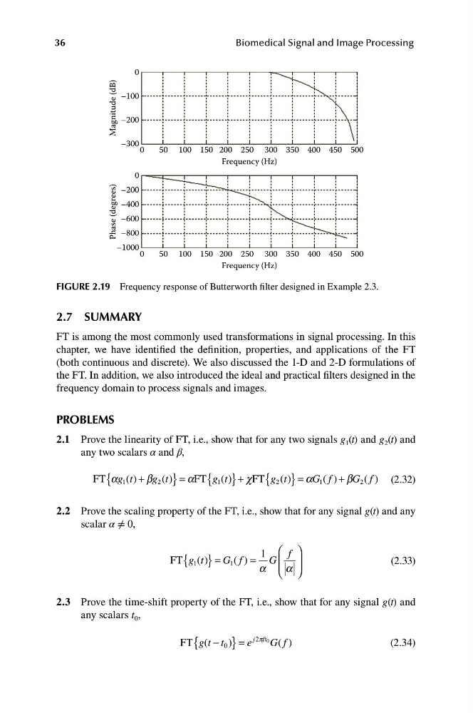
FIGURE 2.19 Frequency response of Butterworth filter designed in Example 2.3.
2.7 SUMMARY
FT is among the most commonly used transformations in signal processing. In this
chapter, we have identified the definition, properties, and applications of the FT
(both continuous and discrete). We also discussed the 1-D and 2-D formulations of
the FT. In addition, we also introduced the ideal and practical filters designed in the
frequency domain to process signals and images.
PROBLEMS
2.1 Prove the linearity of FT, i.e., show that for any two signals g 1 (t) and g 2 (t) and
any two scalars α and β,
FT{ag t
1 ( ) + bg t
2 ( )} = aFT g t
1 ( )} + cFT{g t
( )} = aG f
1 ( ) + bG f
( ) (2.32)
{
2
2
2.2 Prove the scaling property of the FT, i.e., show that for any signal g(t) and any
scalar α ≠ 0,
1
f ⎟ ⎟
FT g t
( )} = G f
⎛ ⎞
{ 1
1 ( ) = G ⎜ ⎜
(2.33)
a
a
⎝ ⎠
2.3 Prove the time-shift property of the FT, i.e., show that for any signal g(t) and
any scalars t 0 ,
2p t 0
FT{g t t
( − 0 )} = e
j f G f
(2.34)
( )
Biomedical Signal and Image Processing
0
–100
–200
–300
Magnitude (dB)
0
50 100 150 200 250 300 350 400 450 500
Frequency (Hz)
0
50 100 150 200 250 300 350 400 450 500
Frequency (Hz)
0
–400
–200
–600
–1000
–800
Phase (degrees)
FIGURE 2.19 Frequency response of Butterworth filter designed in Example 2.3.
2.7 SUMMARY
FT is among the most commonly used transformations in signal processing. In this
chapter, we have identified the definition, properties, and applications of the FT
(both continuous and discrete). We also discussed the 1-D and 2-D formulations of
the FT. In addition, we also introduced the ideal and practical filters designed in the
frequency domain to process signals and images.
PROBLEMS
2.1 Prove the linearity of FT, i.e., show that for any two signals g 1 (t) and g 2 (t) and
any two scalars α and β,
FT{ag t
1 ( ) + bg t
2 ( )} = aFT g t
1 ( )} + cFT{g t
( )} = aG f
1 ( ) + bG f
( ) (2.32)
{
2
2
2.2 Prove the scaling property of the FT, i.e., show that for any signal g(t) and any
scalar α ≠ 0,
1
f ⎟ ⎟
FT g t
( )} = G f
⎛ ⎞
{ 1
1 ( ) = G ⎜ ⎜
(2.33)
a
a
⎝ ⎠
2.3 Prove the time-shift property of the FT, i.e., show that for any signal g(t) and
any scalars t 0 ,
2p t 0
FT{g t t
( − 0 )} = e
j f G f
(2.34)
( )