

30
Biomedical Signal and Image Processing
8
6
4
60
70
80
90 100
Time signal
2
0
–2
–4
–6
0
10
20
30
40
50
Time
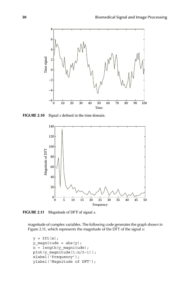
FIGURE 2.10 Signal x defined in the time domain.
140
120
100
30
35
40
45
50
Frequency
Magnitude of DFT
80
60
40
20
0
0
5
10
15
20
25
FIGURE 2.11 Magnitude of DFT of signal x.
magnitude of complex variables. The following code generates the graph shown in
Figure 2.11, which represents the magnitude of the DFT of the signal x:
y = fft(x);
y_magnitude = abs(y);
n = length(y_magnitude);
plot(y_magnitude(1:n/2−1) );
xlabel(‘Frequency’);
ylabel(‘Magnitude of DFT’);
Biomedical Signal and Image Processing
8
6
4
60
70
80
90 100
Time signal
2
0
–2
–4
–6
0
10
20
30
40
50
Time
FIGURE 2.10 Signal x defined in the time domain.
140
120
100
30
35
40
45
50
Frequency
Magnitude of DFT
80
60
40
20
0
0
5
10
15
20
25
FIGURE 2.11 Magnitude of DFT of signal x.
magnitude of complex variables. The following code generates the graph shown in
Figure 2.11, which represents the magnitude of the DFT of the signal x:
y = fft(x);
y_magnitude = abs(y);
n = length(y_magnitude);
plot(y_magnitude(1:n/2−1) );
xlabel(‘Frequency’);
ylabel(‘Magnitude of DFT’);