

29
Fourier Transform
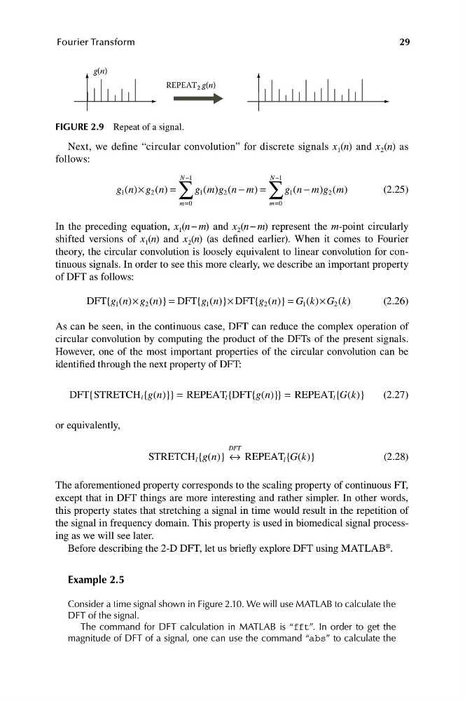
g(n)
REPEAT 2 g(n)
FIGURE 2.9 Repeat of a signal.
Next, we define “circular convolution” for discrete signals x 1 (n) and x 2 (n) as
follows:
∑
N −1
N −1
g 1 ( )
n × g n
2 ( ) =
g 1 (m) g n
2 ( − m) = ∑
g 1 ( n − m)g m
2 ( )
(2.25)
m=0
m=0
In the preceding equation, x 1 (n − m) and x 2 (n − m) represent the m-point circularly
shifted versions of x 1 (n) and x 2 (n) (as defined earlier). When it comes to Fourier
theory, the circular convolution is loosely equivalent to linear convolution for continuous signals. In order to see this more clearly, we describe an important property
of DFT as follows:
DFT{ g n
1 ( ) × g 2 ( n )} = DFT { g n
1 ( )} × DFT {g 2 (n )} = G 1 (k ) × G 2 (k )
(2.26)
As can be seen, in the continuous case, DFT can reduce the complex operation of
circular convolution by computing the product of the DFTs of the present signals.
However, one of the most important properties of the circular convolution can be
identified through the next property of DFT:
DFT {STRETCH l { g n
( )}} = REPEAT l { DFT { g n
( )}} = REPEAT l { G( k )}
(2.27)
or equivalently,
DFT
STRETCH l { g n
( )} ↔ REPEAT l { G( k )}
(2.28)
The aforementioned property corresponds to the scaling property of continuous FT,
except that in DFT things are more interesting and rather simpler. In other words,
this property states that stretching a signal in time would result in the repetition of
the signal in frequency domain. This property is used in biomedical signal processing as we will see later.
Before describing the 2-D DFT, let us briefly explore DFT using MATLAB ® .
Example 2.5
Consider a time signal shown in Figure 2.10. We will use MATLAB to calculate the
DFT of the signal.
The command for DFT calculation in MATLAB is “fft”. In order to get the
magnitude of DFT of a signal, one can use the command “abs” to calculate the
Fourier Transform
g(n)
REPEAT 2 g(n)
FIGURE 2.9 Repeat of a signal.
Next, we define “circular convolution” for discrete signals x 1 (n) and x 2 (n) as
follows:
∑
N −1
N −1
g 1 ( )
n × g n
2 ( ) =
g 1 (m) g n
2 ( − m) = ∑
g 1 ( n − m)g m
2 ( )
(2.25)
m=0
m=0
In the preceding equation, x 1 (n − m) and x 2 (n − m) represent the m-point circularly
shifted versions of x 1 (n) and x 2 (n) (as defined earlier). When it comes to Fourier
theory, the circular convolution is loosely equivalent to linear convolution for continuous signals. In order to see this more clearly, we describe an important property
of DFT as follows:
DFT{ g n
1 ( ) × g 2 ( n )} = DFT { g n
1 ( )} × DFT {g 2 (n )} = G 1 (k ) × G 2 (k )
(2.26)
As can be seen, in the continuous case, DFT can reduce the complex operation of
circular convolution by computing the product of the DFTs of the present signals.
However, one of the most important properties of the circular convolution can be
identified through the next property of DFT:
DFT {STRETCH l { g n
( )}} = REPEAT l { DFT { g n
( )}} = REPEAT l { G( k )}
(2.27)
or equivalently,
DFT
STRETCH l { g n
( )} ↔ REPEAT l { G( k )}
(2.28)
The aforementioned property corresponds to the scaling property of continuous FT,
except that in DFT things are more interesting and rather simpler. In other words,
this property states that stretching a signal in time would result in the repetition of
the signal in frequency domain. This property is used in biomedical signal processing as we will see later.
Before describing the 2-D DFT, let us briefly explore DFT using MATLAB ® .
Example 2.5
Consider a time signal shown in Figure 2.10. We will use MATLAB to calculate the
DFT of the signal.
The command for DFT calculation in MATLAB is “fft”. In order to get the
magnitude of DFT of a signal, one can use the command “abs” to calculate the