

27
Fourier Transform
from the discrete signal, then we could claim that no information has been lost from
the continuous signal. However, it seems impossible to reconstruct the exact values
between the sampled values since there might be several possible options for each
intermediate point. The key issue to address lies on “How fast can a continuous
signal be sampled?”
A theorem called Nyquist or Shannon theorem addresses our problem. The mathematical details and proof of the theorem will not be given here. However, the practical procedure introduced by the theorem for sampling a continuous signal while
maintaining all information in the resulting discrete signal is described in the following steps:
Step 1: Calculate FT of the continuous signal.
Step 2: Find maximum frequency of the signal, i.e., maximum frequency at
which the FT of the signal is nonzero. Call this frequency f M .
Step 3: Sample the continuous signal with a sampling frequency f S , which is
at least twice of f M , i.e., f S ≥ 2f M . In other words, take samples of the continuous signal every T S ≤ 1/2f M s, i.e., sample the continuous signal with a
period that is slower than 1/2f M s.
The rate 2f M that landmarks the slowest sampling rate allowed is called “Nyquist
rate.” The aforementioned theorem states that, if the sampling rate is faster than
Nyquist rate (as indicated in the previous procedure), then the exact continuous signal can be reconstructed from the discrete signal, and, therefore, the resulting discrete signal will contain all details of the continuous signal.
2.4 ONE-DIMENSIONAL DISCRETE FOURIER TRANSFORM
Now that we know how to intelligently sample a continuous signal to preserve all
the information in it, it is time to describe the discrete equivalent of the continuous
FT, called discrete Fourier transform (DFT). Consider a discrete signal g(n), where
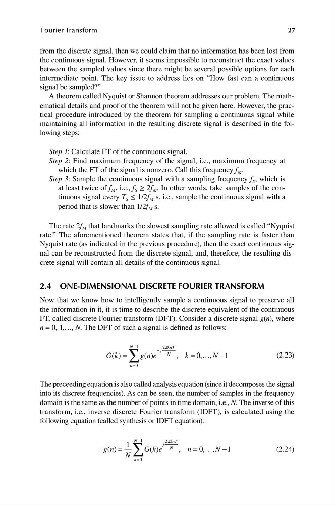
n = 0, 1,…, N. The DFT of such a signal is defined as follows:
N −1
2pknT
G k = ∑
− j
( )
g(n) e N , k = 0 ,…, N −1
(2.23)
n=0
The preceeding equation is also called analysis equation (since it decomposes the signal
into its discrete frequencies). As can be seen, the number of samples in the frequency
domain is the same as the number of points in time domain, i.e., N. The inverse of this
transform, i.e., inverse discrete Fourier transform (IDFT), is calculated using the
following equation (called synthesis or IDFT equation):
1
N −1
2pknT
j
g n
( ) = ∑ G k e
( ) N , n = 0 ,…, N −1
(2.24)
N k =0
Fourier Transform
from the discrete signal, then we could claim that no information has been lost from
the continuous signal. However, it seems impossible to reconstruct the exact values
between the sampled values since there might be several possible options for each
intermediate point. The key issue to address lies on “How fast can a continuous
signal be sampled?”
A theorem called Nyquist or Shannon theorem addresses our problem. The mathematical details and proof of the theorem will not be given here. However, the practical procedure introduced by the theorem for sampling a continuous signal while
maintaining all information in the resulting discrete signal is described in the following steps:
Step 1: Calculate FT of the continuous signal.
Step 2: Find maximum frequency of the signal, i.e., maximum frequency at
which the FT of the signal is nonzero. Call this frequency f M .
Step 3: Sample the continuous signal with a sampling frequency f S , which is
at least twice of f M , i.e., f S ≥ 2f M . In other words, take samples of the continuous signal every T S ≤ 1/2f M s, i.e., sample the continuous signal with a
period that is slower than 1/2f M s.
The rate 2f M that landmarks the slowest sampling rate allowed is called “Nyquist
rate.” The aforementioned theorem states that, if the sampling rate is faster than
Nyquist rate (as indicated in the previous procedure), then the exact continuous signal can be reconstructed from the discrete signal, and, therefore, the resulting discrete signal will contain all details of the continuous signal.
2.4 ONE-DIMENSIONAL DISCRETE FOURIER TRANSFORM
Now that we know how to intelligently sample a continuous signal to preserve all
the information in it, it is time to describe the discrete equivalent of the continuous
FT, called discrete Fourier transform (DFT). Consider a discrete signal g(n), where
n = 0, 1,…, N. The DFT of such a signal is defined as follows:
N −1
2pknT
G k = ∑
− j
( )
g(n) e N , k = 0 ,…, N −1
(2.23)
n=0
The preceeding equation is also called analysis equation (since it decomposes the signal
into its discrete frequencies). As can be seen, the number of samples in the frequency
domain is the same as the number of points in time domain, i.e., N. The inverse of this
transform, i.e., inverse discrete Fourier transform (IDFT), is calculated using the
following equation (called synthesis or IDFT equation):
1
N −1
2pknT
j
g n
( ) = ∑ G k e
( ) N , n = 0 ,…, N −1
(2.24)
N k =0