

δ(t – t 0 )
t 0
t
19
Fourier Transform
Other useful properties of the impulse function include the sampling capability of
the impulse function, i.e., for any signal g(t),
+∞
+
∫
0
d ( )
t g( )
t dt =
∫
d ( )
t g( )
t dt = g(0 )
(2.9)
−∞
−
0
Equation 2.9 describes how integration with impulse function can sample the signal
at the origin. One can also imagine a shifted version of an impulse function centered
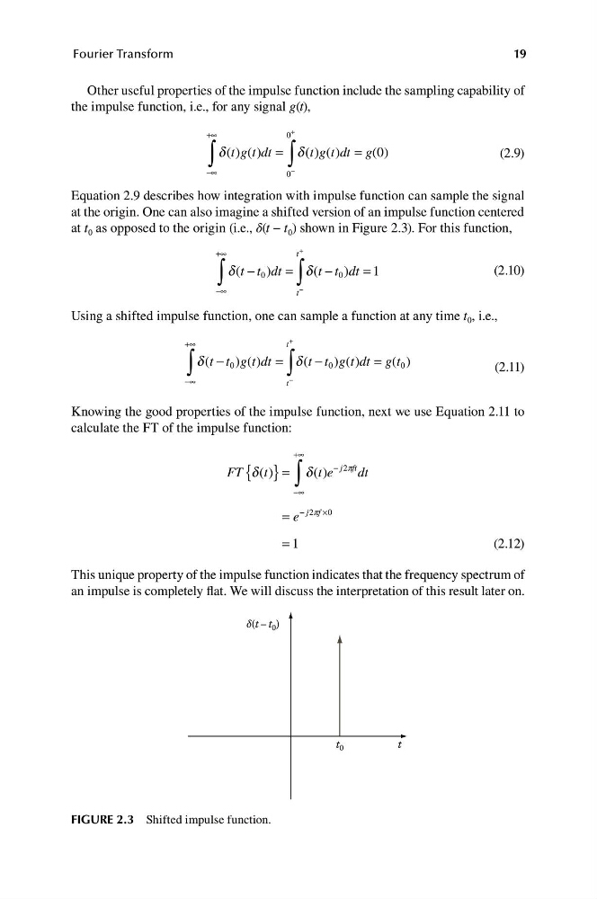
at t 0 as opposed to the origin (i.e., δ(t − t 0 ) shown in Figure 2.3). For this function,
+∞
+
∫
t
d ( t t
− 0 ) dt =
∫
d ( t t
− 0 ) dt = 1
(2.10)
−∞
−
t
Using a shifted impulse function, one can sample a function at any time t 0 , i.e.,
+∞
+
∫
t
d (t − t 0 ) g t
( ) dt =
∫
d (t − t 0 )g t
( ) dt = g t
( 0 )
(2.11)
−∞
−
t
Knowing the good properties of the impulse function, next we use Equation 2.11 to
calculate the FT of the impulse function:
+∞
FT {d ( )
t } = ∫
d ( )
t e
− j f
2 p t dt
−∞
= e
− j f
2p ×0
= 1
(2.12)
This unique property of the impulse function indicates that the frequency spectrum of
an impulse is completely flat. We will discuss the interpretation of this result later on.
FIGURE 2.3 Shifted impulse function.
t 0
t
19
Fourier Transform
Other useful properties of the impulse function include the sampling capability of
the impulse function, i.e., for any signal g(t),
+∞
+
∫
0
d ( )
t g( )
t dt =
∫
d ( )
t g( )
t dt = g(0 )
(2.9)
−∞
−
0
Equation 2.9 describes how integration with impulse function can sample the signal
at the origin. One can also imagine a shifted version of an impulse function centered
at t 0 as opposed to the origin (i.e., δ(t − t 0 ) shown in Figure 2.3). For this function,
+∞
+
∫
t
d ( t t
− 0 ) dt =
∫
d ( t t
− 0 ) dt = 1
(2.10)
−∞
−
t
Using a shifted impulse function, one can sample a function at any time t 0 , i.e.,
+∞
+
∫
t
d (t − t 0 ) g t
( ) dt =
∫
d (t − t 0 )g t
( ) dt = g t
( 0 )
(2.11)
−∞
−
t
Knowing the good properties of the impulse function, next we use Equation 2.11 to
calculate the FT of the impulse function:
+∞
FT {d ( )
t } = ∫
d ( )
t e
− j f
2 p t dt
−∞
= e
− j f
2p ×0
= 1
(2.12)
This unique property of the impulse function indicates that the frequency spectrum of
an impulse is completely flat. We will discuss the interpretation of this result later on.
FIGURE 2.3 Shifted impulse function.