

12
Biomedical Signal and Image Processing
number of pixels in the image whose gray level equals r and name it as n(r). Then,
we divide that number by the total number of points in the image n, i.e.,
n r
( )
p r
( ) =
(1.1)
n
The reason for using p(r) to represent these normalized frequencies is due to the fact
that in limit these frequencies approach the true probabilities of gray levels. Then,
histogram is defined as the graph of p(r) versus r. The definition of this concept is
illustrated in the following examples.
Example 1.2
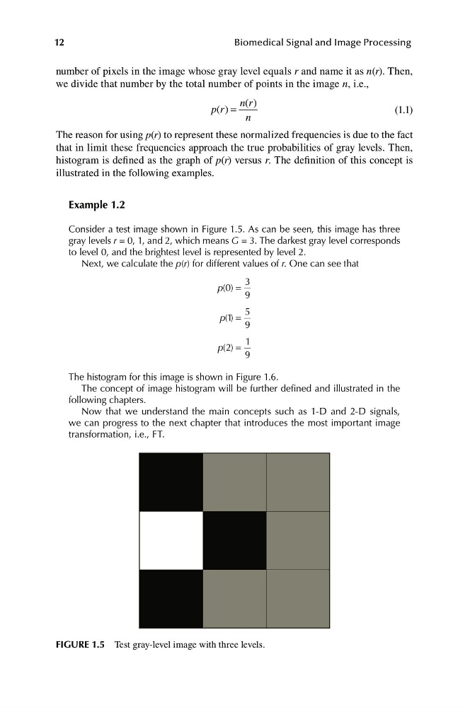
Consider a test image shown in Figure 1.5. As can be seen, this image has three
gray levels r = 0, 1, and 2, which means G = 3. The darkest gray level corresponds
to level 0, and the brightest level is represented by level 2.
Next, we calculate the p(r) for different values of r. One can see that
3
p( ) =
0
9
5
p( )
1 =
9
1
p( ) =
2
9
The histogram for this image is shown in Figure 1.6.
The concept of image histogram will be further defined and illustrated in the
following chapters.
Now that we understand the main concepts such as 1-D and 2-D signals,
we can progress to the next chapter that introduces the most important image
transformation, i.e., FT.
FIGURE 1.5 Test gray-level image with three levels.
Biomedical Signal and Image Processing
number of pixels in the image whose gray level equals r and name it as n(r). Then,
we divide that number by the total number of points in the image n, i.e.,
n r
( )
p r
( ) =
(1.1)
n
The reason for using p(r) to represent these normalized frequencies is due to the fact
that in limit these frequencies approach the true probabilities of gray levels. Then,
histogram is defined as the graph of p(r) versus r. The definition of this concept is
illustrated in the following examples.
Example 1.2
Consider a test image shown in Figure 1.5. As can be seen, this image has three
gray levels r = 0, 1, and 2, which means G = 3. The darkest gray level corresponds
to level 0, and the brightest level is represented by level 2.
Next, we calculate the p(r) for different values of r. One can see that
3
p( ) =
0
9
5
p( )
1 =
9
1
p( ) =
2
9
The histogram for this image is shown in Figure 1.6.
The concept of image histogram will be further defined and illustrated in the
following chapters.
Now that we understand the main concepts such as 1-D and 2-D signals,
we can progress to the next chapter that introduces the most important image
transformation, i.e., FT.
FIGURE 1.5 Test gray-level image with three levels.